Accelerator and Heavy Flavor Physics – Introductory Concepts

Introduction

In this post, we delve into the primary field of focus of this text: high-energy particle physics. We begin by introducing fundamental concepts in accelerator physics, followed by an overview of the Standard Model (SM) and some key open questions in the field. Finally, we touch on heavy flavor physics in a bit more detail. This background will be necessary to understand and precisely describe the work from the physics point of view.

Accelerator Physics

Cylindrical Coordinates

In accelerator physics, cylindrical coordinates \((\rho, \varphi, z)\) [Ref] are often used, instead of Cartesian coordinates \((x,y,z)\). In this configuration, points are identified with respect to the main axis called cylindrical or longitudinal axis, and an auxiliary axis called the polar axis, as shown in Fig. 1. \(\rho\) denotes the perpendicular distance from the main axis, \(z\) denotes the distance along the main axis, and \(\varphi\) is the plane (or azimuthal) angle of the point of projection on the transverse plane. The beamline is naturally identified with the cylindrical axis of the coordinate system.

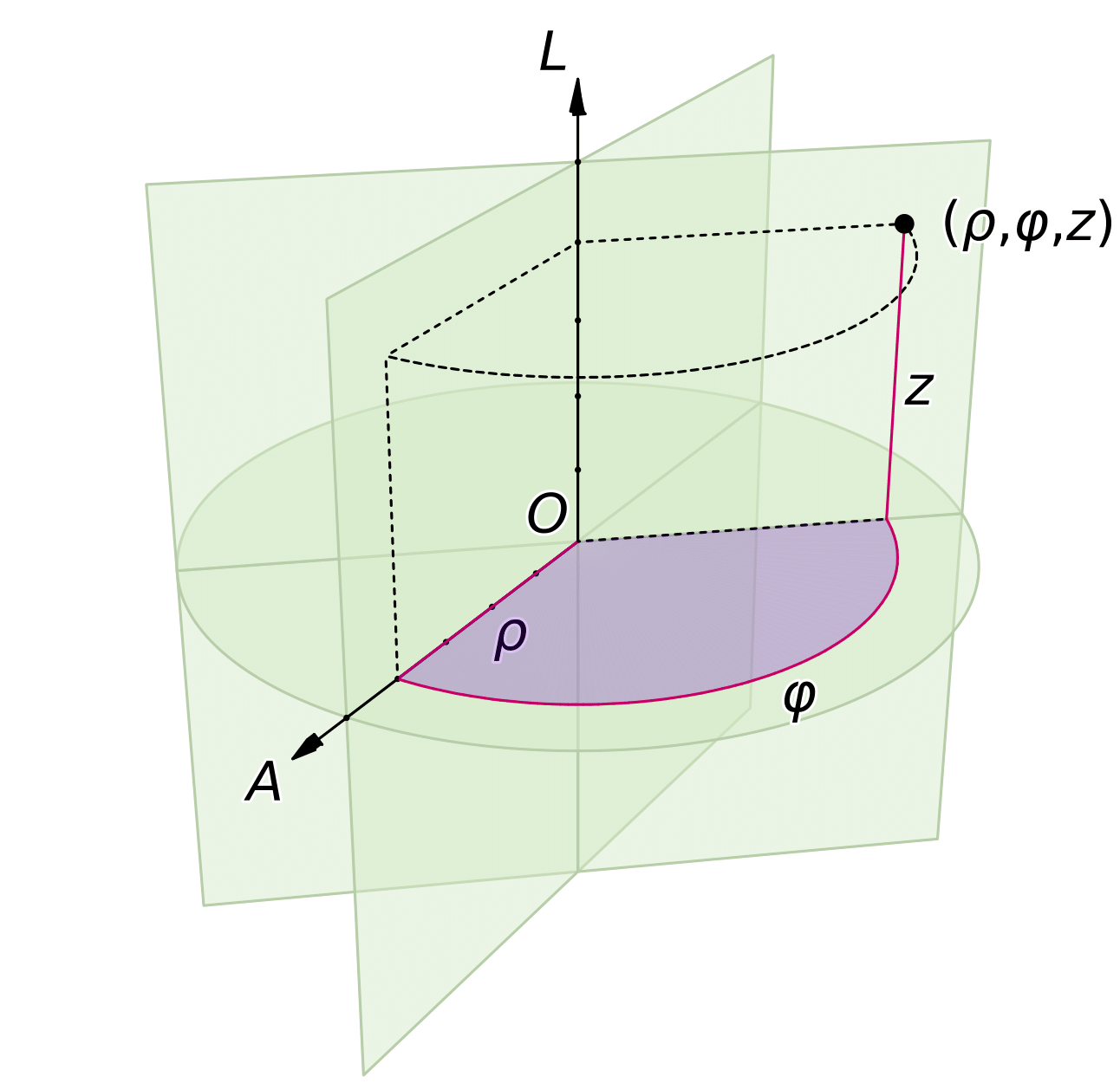
Figure 1: A cylindrical coordinate system defined by an origin \(O\), a polar (radial) axis \(A\), and a longitudinal (axial) axis \(L\). Figure from [Ref].

Pseudorapidity

In experimental particle physics, another frequently used spatial coordinate is the pseudorapidity \(\eta\) . It describes the angle between a particle’s momentum \(\mathbf{p}\) and the positive direction of the beam axis—identified with the \(z\)-direction. This angle is referred to as the polar angle \(\theta\), as shown in Fig. 2.

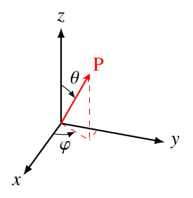
Figure 2: The polar (\(\theta\)) and azimuthal (\(\varphi\)) angles. Adapted from [Ref].

Pseudorapidity is defined as [Ref]:

\[ \eta = - \ln \left[ \tan \left( \frac{\theta}{2} \right) \right]\,, \] or inversely

\[ \theta = 2 \arctan \left( e^{-\eta}\right) \,. \] As a function of the three-momentum \(\mathbf{p}\), pseudorapidity can be expressed as

\[ \eta = \frac{1}{2} \ln \left( \frac{|\mathbf{p}| + p_L}{|\mathbf{p}| - p_L} \right)\, \] where \(p_L\) is the longitudinal component of the momentum, along the beam axis. Due to its desirable physical properties, this definition is highly favored in experimental particle physics.

From the above equation, we can see that when the momentum tends to be all along the beamline, i.e., \(p_L \rightarrow \lvert \mathbf{p} \rvert \) (\(\theta \rightarrow 0 \)), pseudorapidity blows up \(\eta \rightarrow \infty \). On the other hand, when most of the momentum is in transverse directions, \(p_L \rightarrow 0 \) (\(\theta \rightarrow 90^{\circ} \)), then \(\eta \rightarrow 0 \), as shown in Fig. 3.

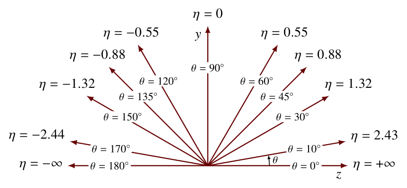
Figure 3: Values of pseudorapidity \(\eta\) versus polar angle \(\theta\). Figure from [Ref].

Beam Bunching

In particle beams, in many modern experiments including the LHC, particles are distributed into pulses, or bunches. Bunched beams are common because most modern accelerators require bunching for acceleration [Ref].

At the LHC, after accelerating the particles in bunches, the two beams are focused resulting in the crossing of these bunches—the so-called bunch crossing, as shown in Fig. 4. These bunch crossings, also known as events, may result in one or multiple collisions between protons and consequently in the production of new particles. The number of these collisions during a bunch crossing is known as pile-up.

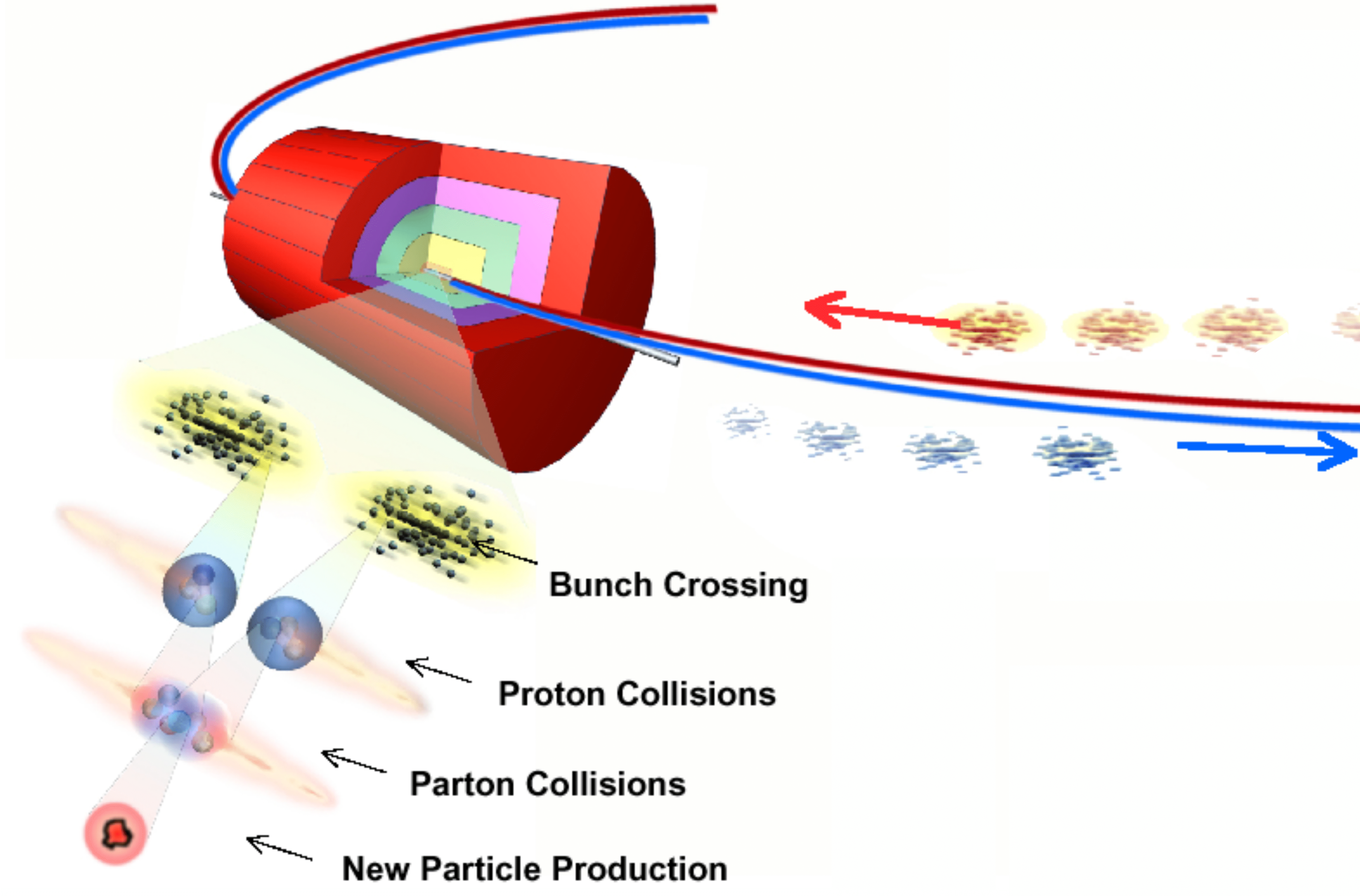
Figure 4: Illustration of beam bunching utilized at the Large Hadron Collider at CERN. Adapted from [Ref].

Primary and Secondary Vertices

Primary vertices are points in space where a particle collision occurred, resulting in the generation of other particles at this point, as shown in Fig. 5. The location of this point can be reconstructed from the tracks of particles emerging directly from the collision. Secondary (or displaced) vertices are points displaced from the primary vertex, where the decay of a long-lived particle occurred. These points can be reconstructed from the tracks of decay products that do not originate from the primary interaction.

Primary vertices are a crucial element of many physics analyses [Ref]. The precise reconstruction of many processes, the identification of \(b\)- or \(\tau\)-jets, the reconstruction of exclusive \(b\)-decays and the measurement of lifetimes of long-lived particles are all dependent upon the precise knowledge of the location of the primary vertex. Secondary vertices, on the other hand, are tools for identifying heavy flavor hadrons and \(\tau\) leptons [Ref].

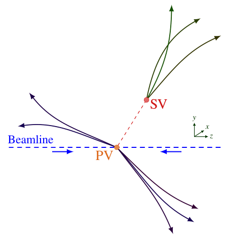
Figure 5: Illustration of Primary Vertices (PVs) and Secondary Vertices (SVs) in colliding-beam experiments. PVs are points in space where a primary particle collision occurred, and can reconstructed from the tracks of particles emerging directly from the collision. SVs, on the other hand, are points displaced from the PV where the decay of a long-lived particle occurred. They can be reconstructed from the tracks of decay products that do not originate from the primary interaction. Adapted from [Ref].

Luminosity

Luminosity \(L\) is defined as the ratio of the number of events detected \(dN\) in a certain period of time \(dt\) and across a cross section \(\sigma\) [Ref]:

\[ L = \frac{1}{\sigma} \frac{dN}{dt} \,, \] and is often given units of \(\text{cm}^{-2} \cdot \text{s}^{-1}\). In practice, the luminosity depends on the parameters of the particle beam, such as the beam width and particle flow rate.

Integrated luminosity \(L_{\text{int}}\) is defined as the integral of the luminosity with respect to time:

\[ L_{\text{int}} = \int L \,dt = \frac{N}{\sigma} \,, \] where \(N\) is now the total number of collision events produced. \(L\) is frequently referred to as instantaneous luminosity, in order to emphasize the distinction between its integrated-over-time counterpart \(L_{\text{int}}\). Integrated luminosity, having units of \(1/\sigma\), is sometimes measured in inverse femtobarns \(\text{fb}^{-1}\). It measures the number of collisions produced per femtobarn of cross section.

These variables are useful quantities to evaluate the performance of a particle accelerator. In particular, most HEP collision experiments aim to maximize their luminosity, since a higher luminosity means more collisions and consequently a higher integrated luminosity means a larger volume of data available to be analyzed.

For beam-to-beam experiments, where the particles are accelerated in opposite directions before collided, like the majority of the time at the LHC, the instantaneous luminosity can be calculated as [Ref]:

\[ L = \frac{N^2 f N_b}{4 \pi \sigma_x \sigma_y} \,, \] where \(N\) denotes the number of particles per bunch, \(f\) is the revolution frequency, and \(N_b\) is the number of bunches in each beam. The transverse dimensions of the beam, assuming a Gaussian profile, are described by \(\sigma_x\) and \(\sigma_y\).

Impact Parameter

The impact parameter \(b\) represents the shortest, perpendicular distance between the trajectory of a projectile and the center of the potential field generated by the target particle, as shown in Fig. 6. In accelerator experiments, collisions can be classified based on the value of the impact parameter. Central collisions have \(b \approx 0\), while peripheral collisions have impact parameters comparable to the radii of the colliding nuclei.

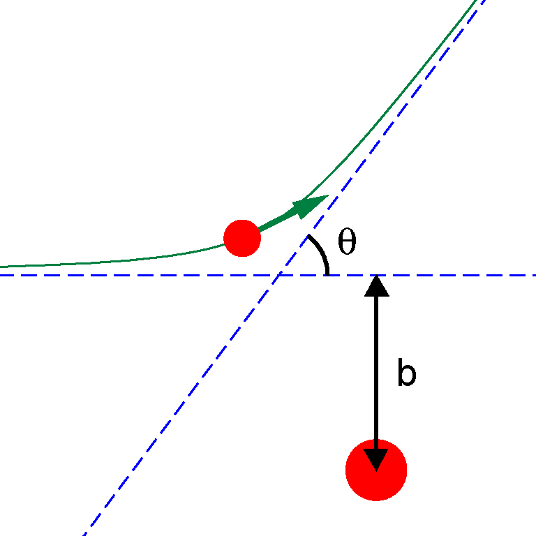
Figure 6: A projectile scattering off a target particle. The impact parameter \(b\) and the scattering angle \(\theta\) are shown. Figure from [Ref].

Detector Acceptance

In particle collider experiments, the location of the collisions is predetermined. However, the direction of the produced particles due to the interactions is not predetermined, i.e., the products can fly in every possible direction. However, depending on the geometry of the experiment or its physics program, detecting all the products is not feasible or desirable. The region of the detector where the particles are in fact detectable is referred to as the acceptance. In some cases, detection depends also on the energy, or other characteristics of the particle, meaning that the acceptance is not only a function of the particle’s direction, but also of those extra characteristics.

The Standard Model of Particle Physics

The SM is a relativistic quantum field theory classifying all known elementary particles and describing three out of the four fundamental forces: the electromagnetic, weak nuclear and strong nuclear interactions, excluding gravity. It was developed progressively during the latter half of the 20th century through the contributions of numerous scientists worldwide [Ref]. Its current form was established in the mid-1970s following the experimental confirmation of quarks. Subsequent discoveries, including the top quark in 1995 [Ref], the tau neutrino in 2000 [Ref], and the Higgs boson in 2012 [Ref], have further reinforced the validity of the Standard Model.

Fig. 7 depicts the elementary particles of the SM and their interactions. They can be divided into twelve fermions with spin-\(1/2\), five spin-1 gauge bosons (\(\gamma, g^a, W^{\pm}, Z^0\)), carriers of the electromagnetic, weak and strong interactions, and the spin-0 (scalar) Higgs boson (\(H\)).

The fermions are further grouped into six quarks and six leptons. The main difference is that quarks interact with all three fundamental forces of the SM, while leptons only interact with the weak and electromagnetic interactions. Quarks appear in six different flavors. In increasing order of quark masses they are called: up (\(u\)), down (\(d\)), strange (\(s\)), charm (\(c\)), bottom or beauty (\(b\)) and top (\(t\)) quarks. The quarks are further grouped into three generations of increasing masses. Up-type quarks (\(u\), \(c\), \(t\)) have an electric charge \(q=+(2/3)e\) while down-type quarks (\(d\), \(s\), \(b\)) have \(q=-(1/3)e\), where \(e\) is the elementary charge.

Quarks possess a property known as color charge, which causes them to interact through the strong force. Due to color confinement, quarks are tightly bound together, forming color-neutral composite particles called hadrons. As a result, quarks cannot exist in isolation and must always combine with other quarks. Hadrons are classified into two types: mesons, which consist of a quark-antiquark pair, such as the pion (\(\pi\)), the kaon (\(K\)), the \(B\), \(D\) and \(J/\psi\) mesons, and baryons, which are made up of three quarks. The lightest baryons are the nucleons: the proton and the neutron.

Furthermore, the solutions of the Dirac equation [Ref] predict that each of the twelve SM fermions has a corresponding counterpart, known as its antiparticle, which possesses the same mass but opposite charge.

Similarly, the leptons are also grouped into three generations. Each generation contains a charged lepton and its corresponding uncharged neutrino. The charged leptons are the electron (\(e^-\)), the muon (\(\mu^-\)) and the tau (\(\tau^-\)). Their uncharged partners are the electron, muon and tau neutrinos (\(\nu_e\), \(\nu_{\mu}\), \(\nu_{\tau}\)). Being chargeless, they are not sensitive to the electromagnetic interaction and moreover, they are considered massless in the SM. The observation of neutrino oscillations [Ref] requires that neutrinos have small but non-zero masses and thus implies physics beyond the SM.

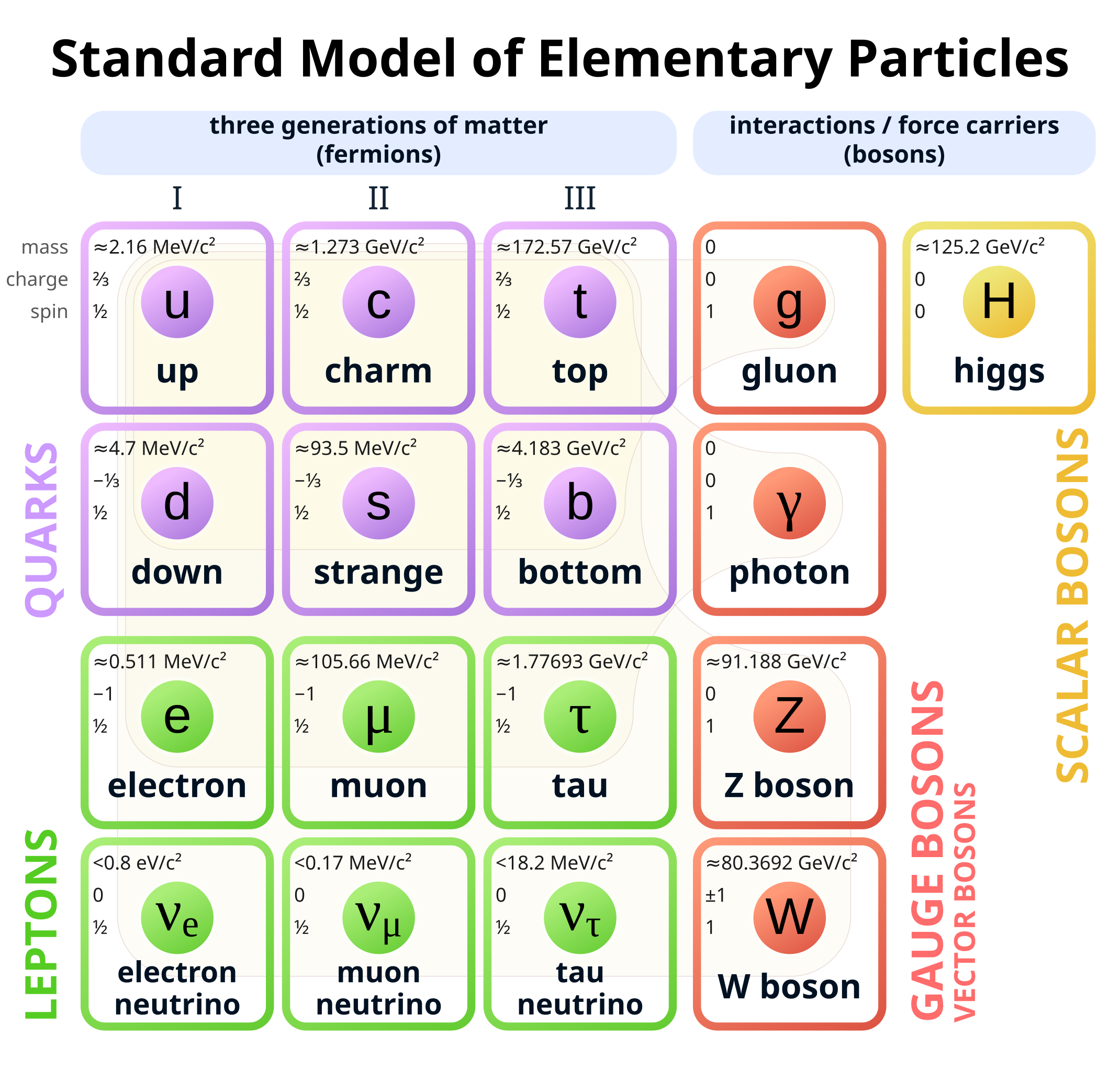
Figure 7: The Standard Model of elementary particles including twelve fundamental fermions and five fundamental bosons. Brown loops indicate the interactions between the bosons (red) and the fermions (purple and green). Please note that the masses of some particles are periodically reviewed and updated by the scientific community. The values shown in this graphic are taken from [Ref]. Figure from [Ref].

The five types of gauge bosons mediate the interactions between the fermions. The electromagnetic is mediated by the photon \(\gamma\), the strong by eight distinct gluons \(g^a\), and the weak by the W\(^{\pm}\) and Z\(^0\) bosons. The Higgs boson plays a special role in the Standard Model by providing an explanation for why elementary particles, except for the photon and gluon, have mass. Specifically, the Higgs mechanism is responsible for the generation of the gauge boson masses while the fermion masses result from Yukawa-type interactions with the Higgs field.

Table 1 summarizes the masses \(m\) and electric charges \(q\) of the fermionic elementary particles of the SM, while in Table 2, the masses, charges and spins of the elementary bosons are shown.

Generation	Quark	\(m\) (MeV/\(c^2\))	\(q\) (\(e\))	Lepton	\(m\) (MeV/\(c^2\))	\(q\) (\(e\))
1	\(u\)	\(2.16 \pm 0.07\)	+2/3	\(\nu_e\)	\(<2 \times 10^{-6}\)	0
	\(d\)	\(4.70 \pm 0.07\)	-1/3	\(e^-\)	0.511	-1
2	\(c\)	\(1273.0 \pm 4.6\)	+2/3	\(\nu_{\mu}\)	\(<0.19\)	0
	\(s\)	\(93.5 \pm 0.8\)	-1/3	\(\mu^-\)	105.66	-1
3	\(t\)	\(172\,570\pm 290\)	+2/3	\(\nu_{\tau}\)	\(<18.2\)	0
	\(b\)	\(4183 \pm 7\)	-1/3	\(\tau^-\)	1777	-1

Table 1: Summary of the masses and charges of the elementary fermions in the SM. Mass values taken from [Ref]. Uncertainties are not displayed for masses if they are smaller than the last digit of the value.

Boson	Type	Spin	\(m\) (GeV/\(c^{2}\))	\(q\) (\(e\))
Photon	Gauge	1	0	0
Gluon	Gauge	1	0	0
Z\(^0\)	Gauge	1	\(91.1880 \pm 0.0020\)	0
W\(^{\pm}\)	Gauge	1	\(80.3692 \pm 0.0133\)	\(\pm 1\)
Higgs	Scalar	0	\(125.20 \pm 0.11\)	0

Table 2: Summary of the masses, charges and spins of the elementary bosons of the SM. Mass values taken from [Ref]. The masses of the photon and the gluon are the theoretical values.

Open Questions

Despite the successes of the Standard Model, it is not a complete theory of fundamental interactions and several questions in physics remain open [Ref]. For example, even though the three out of the four fundamental forces have been combined into the same theory, gravity, described by the general theory of relativity, cannot be integrated into the SM. The problem remains elusive, and theories Beyond the Standard Model (BSM) are needed, such as string theory or quantum gravity. In addition, the question of why there is more matter in the universe than antimatter, remains an open question. This problem is known as the matter-antimatter asymmetry and is a core question in the LHCb physics program. Furthermore, this question is related to CP violation, the violation of the charge-conjugation parity symmetry in particle interactions. This is one of the reasons why CP violation is heavily studied at LHCb. Moreover, it does not account for the accelerating expansion of the universe, and how it is possibly described by dark energy. Finally, the origin of dark matter remains to be understood as well as the explanation for neutrino oscillations and their non-zero masses.

Heavy Flavor Physics

Going into more detail, the gigantic datasets being collected by the various accelerator experiments—and specifically by the Large Hadron Collider beauty (LHCb) experiment—are crucial to shed light on many of the open questions in particle physics [Ref], and in particular in heavy flavor physics.

An important matrix in flavor physics is the so-called Cabibbo–Kobayashi–Maskawa (CKM) matrix [Ref], and is of the form:

\[ V_{CKM} = \] \[ V_{ud}, V_{us} , V_{ub} \] \[ V_{cd} , V_{cs} , V_{cb} \] \[ V_{td} , V_{ts} , V_{tb} \,. \]

It is a unitary matrix that dictates the quark mixing strengths of the flavor-changing weak interaction, and is crucial in understanding CP violation. The unitarity of the CKM matrix imposes constraints on its elements, which can be visualized geometrically through the construction of so-called unitarity triangles. Unitarity triangles have angles conventionally labeled as \(\alpha\), \(\beta\) and \(\gamma\). The angle \(\beta\) is conventionally measured from the mixing-induced CP violation in \(B^0 \to J/\psi K^0_S\) decays. The angle \(\alpha\) is determined using the \(B\to \pi \pi\), \(\pi \rho\) and \(\rho \rho\) decays, while \(\gamma\) is inferred from CP violation effects in \(B^+ \to D K^+\) [Ref]. The angles above are related to the unitarity relation between the rows of the CKM matrix corresponding to the couplings of the \(b\) and \(d\) quarks to \(u\) quarks. The current uncertainties, measured by LHCb, are \(0.57^{\circ}\) [Ref] and \(2.8^{\circ}\) [Ref] for \(\beta\) and \(\gamma\), respectively. These sensitivities have been achieved using data samples of integrated luminosity 2–9 fb\(^{-1}\). These values are projected to be reduced to \(0.20^{\circ}\) and \(0.8^{\circ}\), respectively, with 50 fb\(^{-1}\) of data recorded by the early 2030s, and even to \(0.08^\circ\) and \(0.3^\circ\), respectively, with 300 fb\(^{-1}\) of data recorded by the early 2040s.

Improving our understanding of the CKM matrix through global fits requires more precise knowledge of the magnitudes of the \(\vert V_{ub} \rvert\) and \(\lvert V_{cb}\rvert \) CKM matrix elements. We can determine these magnitudes by studying semileptonic decays like \(b \to u l \nu\) and \(b \to cl \nu\), where \(l\) denotes a charged lepton. Semileptonic decays can also be utilized to test the SM predictions on universality between the charged current weak interactions with different lepton flavors. This can be done using observables such as \(R(D^{(* )})\), which are the branching fraction ratios

\[ \frac{B \to D^{(* )} \tau \nu}{B \to D^{(* )} e \nu} \] or \[ \frac{B \to D^{(* )} \tau \nu}{B \to D^{(* )} \mu \nu} \,. \] The current values of these quantities suggest possible discrepancies with the SM. In order to further explore these discrepancies, the measured uncertainties on these values have to be reduced. Currently, the uncertainty on both \(|V_{ub}|\) [Ref] and \(R(D^{(* )})\) [Ref] is at 6%, from LHCb measurements. These uncertainties are projected to be reduced down to 1% and 3%, for \(|V_{ub}|\) and \(R(D^{(* )})\), respectively, with the increased number of collisions expected until the early 2040s.

Moreover, even though all CP violation in the charm sector is suppressed in the SM, CP violation in \(D^0\)-meson decays has been observed through asymmetries in \(D^0 \to K^+ K^-\) and \(D^0 \to \pi^+ \pi^-\) decays, captured by the observable \(\Delta A_{CP} = A_{CP}\left(D^0 \to K^+ K^- \right) - A_{CP}\left(D^0 \to \pi^+ \pi^- \right)\). \(A_{CP}(D^0 \to f)\) denotes the asymmetry between the \(D^0 \to f\) and \(\bar{D}^0 \to f\) decay rates to a final state \(f\). With a sample of 5.9 fb\(^{-1}\), LHCb quoted an uncertainty of \(29 \times 10^{-5}\) [Ref]. This uncertainty can be potentially reduced almost by a factor of 10, down to \(3.3 \times 10^{-5}\), given the expected integrated luminosities of 300 fb\(^{-1}\). Furthermore, the charm samples essential to these measurements are produced at very large signal rates. Without real-time processing at the full collision rate these samples would be impossible to collect.

Beyond CP violation, the study of lepton flavor violation offers another compelling avenue for discovering BSM physics. While lepton flavor violation occurs in neutrino oscillations, any related effect in charged leptons is unobservably small within the SM framework. Consequently, observing any non-zero effect would be an unambiguous sign of BSM physics. Similarly, stringent upper limits on branching fractions, like \(\mathcal{B}(\tau^+ \to \mu^+ \gamma)\) and \(\mathcal{B}(\tau^+ \to \mu^+ \mu^+ \mu^-)\), tightly constrain potential BSM extensions of the Standard Model. For example, with a data sample of 424 fb\(^{-1}\), the Belle II collaboration has constrained \(\mathcal{B}(\tau^+ \to \mu^+ \mu^+ \mu^-)\) down to \(<1.8 \times 10^{-8}\) [Ref]. This uncertainty, using 50 ab\(^{-1}\) instead, is projected to be reduced down to \(<0.02 \times 10^{-8}\) until the early 2040s.

Heavy flavor physics remains a vital part of the global particle physics program. While experiments including ATLAS, CMS, LHCb and Belle II offer complementary strengths, they will also compete for the best precision on certain observables. This competion will allow for crucial consistency checks and ultimately lead to even more precise world average combinations. Collectively, these experiments can significantly advance the experimental precisions of all the key observables in \(b\), \(c\) and \(\tau\) physics, with an expected improvement of typically one order of magnitude from what is available today. Nonetheless, this represents only a partial evaluation of the true physics reach, suggesting the impact will probably be even more significant. The precision currently at reach with these experiments, including their upgrades, provides an unprecedented capability to probe the flavor sector of the Standard Model.

Conclusion

In this post, I started by introducing fundamental concepts in accelerator physics, necessary to understand the technical aspects related to the detector physics of this work. I also described the Standard Model of particle physics, the open questions in the field, and finally the research outlook and expected impact of heavy flavor physics research.

This article is one of the chapters of my PhD thesis titled: “Real-Time Analysis of Unstructured Data with Machine Learning on Heterogeneous Architectures”. The full text can be found here: PhD Thesis. In the main results part of this work, GNNs were used to perform the task of track reconstruction, in the context of the Large Hadron Collider (LHC) at CERN.