From Machine Learning to Graph Neural Networks and Quantization – An Introduction

Introduction

This post is a short and pedagogical introduction to the field of Machine Learning (ML) and its brief history, its subfields Deep Learning (DL) and Graph Neural Networks (GNNs), as well as some important techniques highly relevant to the field of ML and the deployment of ML models in high-throughput or resource-constrained contexts.

Parts of this text were inspired by [Ref] and [Ref].

Machine Learning

Machine learning is the field of how machines—specifically computers—can “learn”. Although “learn” is perhaps a generous term, it refers to how computers manage to do specific tasks without being explicitly programmed to do them. Unlike classical algorithms, which follow hand-crafted rules defined by developers, ML algorithms, and by consequence ML models, are data-driven: By an iterative process of providing data to the ML model, the model is trained and progressively learns to perform a task solely based on the data it has been given. At the end of this process, without the need for the developer to describe the logic of the algorithm itself, the model can carry out the task effectively without the developer needing to explicitly define how it should be done.

The term machine learning is believed to have been coined by Arthur Samuel in 1959 for his work on programming a computer to play checkers [Ref]. In general, Artificial Intelligence (AI) is considered as a more general term than ML, as shown in Fig. 1. Strictly speaking it refers to the capability of computational systems to mimic tasks which normally require human intelligence, such as learning, reasoning, decision-making, and problem solving. However, the two terms ML and AI are often used interchangeably.

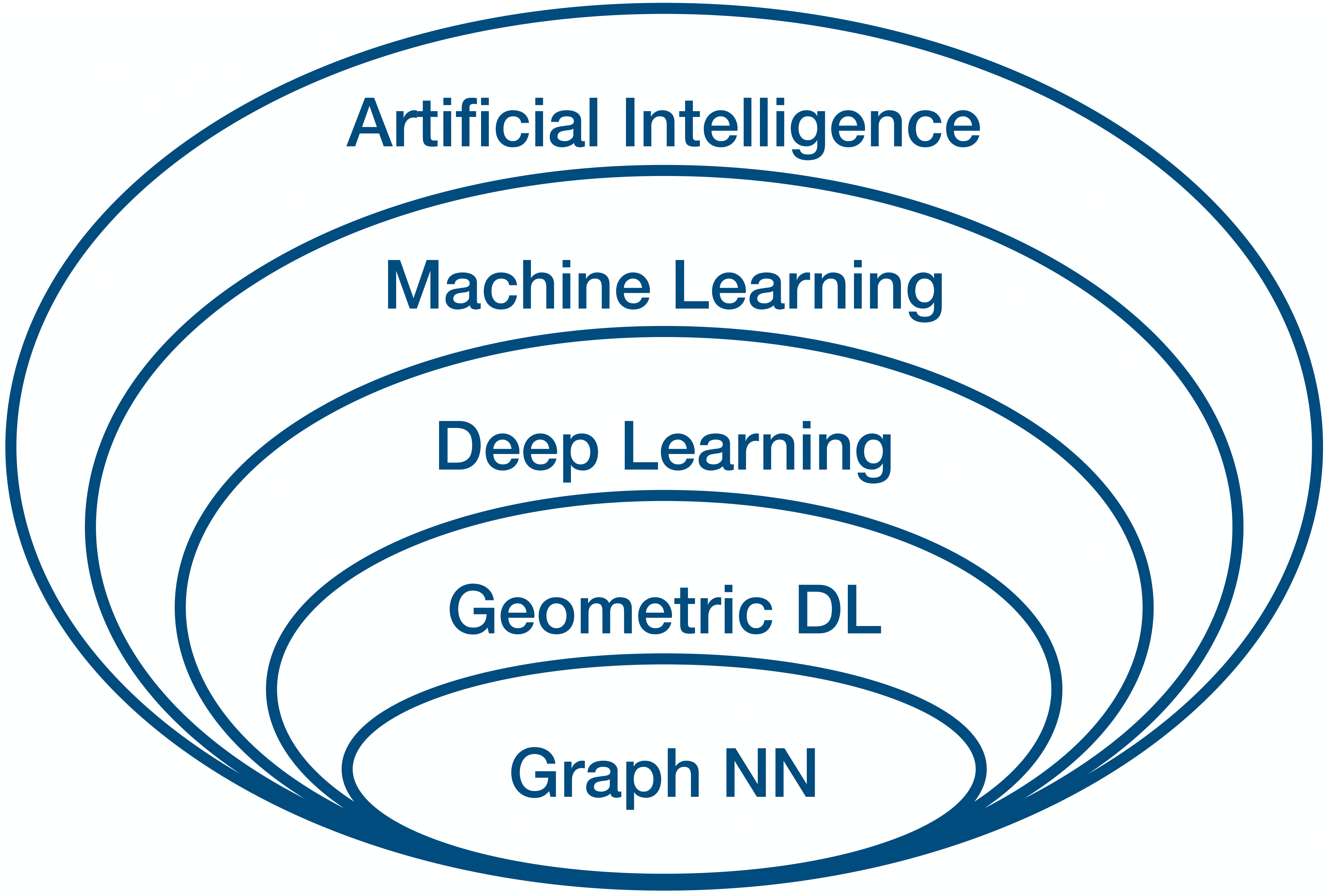
Figure 1: Euler diagram of AI and its subfields as relevant to this post.

Classical, or probabilistic, ML has been in use long before the term ML came into existence. These algorithms are statistical models that try to capture relationships between various variables. Arguably, the most famous example is linear regression, originally developed by Isaac Newton for his work on the equinoxes around 1700 [Ref], and later formalized by Legendre and Gauss in the early 19th century [Ref].

The performance of these simple ML algorithms strongly depends on the representation of the data they are given. For example, as illustrated in Fig. 2, the coordinate system used: Switching from Cartesian to polar coordinates might have a dramatic impact on the performance of an algorithm in solving a specific task. Each piece of information included in the representation of a data class, coordinates \(x \), \(y \) and \(r \), \(\theta \) in our example in Fig. 2, is known as a feature. Linear regression tries to capture the relationship between these features, the independent variables, and the dependent variables. However, it cannot influence our choice for the definition of the features to be used.

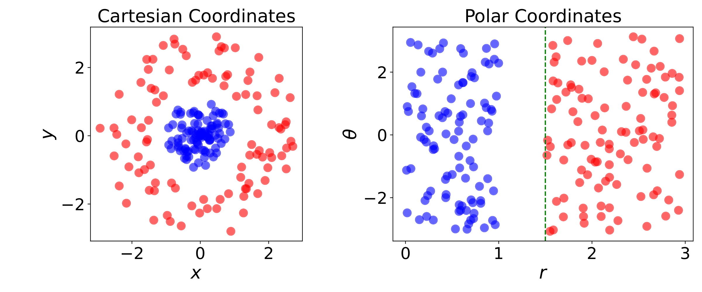
Figure 2: Example of different representations: Suppose we want to separate two classes of data by drawing a line between them. If the data are represented in Cartesian coordinates (left) the task is impossible. On the other hand, when the same points are represented in polar coordinates (right), the task becomes very simple to solve with a vertical separator.

Many ML tasks can be efficiently solved by designing the right set of features for that task, and then providing these features to a simple machine learning algorithm. As an example, imagine we have a set of images of either grass fields or the sea. What feature can we design to separate the two groups of images? We could find the average color of all the pixels and if the average is close to green then we would label the photo as “grass”, while if it is close to blue as “sea”. We can be confident that with this simple feature we have extracted, the performance of our classification algorithm is likely to be adequate for this task.

However, what happens if we pass each photo through a color filter, changing the color of the pixels? In this case, the algorithm breaks down completely. However, to a human eye, the classification task remains identically easy. So, how do we capture the “seaness” of the sea and the “grassness” of the grass? This is exactly where things get difficult. It is not obvious how to design a feature exactly in order to capture, for example, the texture of the grass in terms of pixel values. This is where representation learning, also known as feature learning, comes in. It is a set of techniques that allows a system to automatically discover the representation needed for a specific problem, completely bypassing the need for hand-designing. And as it turns out, learned representations often result in much better performance than hand-designed ones [Ref].

Deep learning is a form of representation learning and involves Neural Networks (NNs) with multiple layers. The NN learns hierarchical representations of data, i.e from low-level (e.g., edges in images) to high-level features (e.g., faces, objects). Frank Rosenblatt is attributed with introducing the perceptron in 1958 [Ref]. Combining multiple of these perceptrons arranged in layers results in the so-called Multilayer Perceptron (MLP), also known as a Feedforward Neural Network (FNN). The first MLP trained by stochastic gradient descent [Ref] was published by Shun’ichi Amari in 1967 [Ref]. The ReLU (Rectified Linear Unit) activation function, introduced in 1969 by Kunihiko Fukushima [Ref], has now become the most popular activation function for deep learning [Ref]. Finally, the modern form of backpropagation was first published in 1970 by Seppo Linnainmaa [Ref]. The method applied to neural networks was popularized by David E. Rumelhart et al. in 1986 [Ref].

During the 1990s, introduced by Yann LeCun [Ref], Convolutional Neural Networks (CNNs) marked a major breakthrough. In his seminal work, he proposed the LeNet-5 architecture, which utilized convolutional layers to recognize hand-written digits from the MNIST database—a significant shift from traditional fully connected layers.

The Revolution

The ML/DL revolution was kick-started by CNN-based computer vision in 2012 [Ref], driven by advancements in computation, particularly the graphics processing unit. Although CNNs trained via backpropagation had existed for decades, and neural networks—including CNNs—had already been implemented on GPUs for years [Ref], advancements in computer vision required faster GPU implementations. At the same time, in 2006, GPUs became programmable with Nvidia’s CUDA framework [Ref]. As deep learning gained widespread adoption, specialized hardware and optimized algorithms were subsequently developed to meet its growing demands [Ref]. In 2009, Rajat Raina et al. demonstrated an early example of GPU-accelerated deep learning by training a 100-million-parameter deep belief network using 30 Nvidia GeForce GTX 280 GPUs [Ref]. Their approach achieved training speeds up to 70 times faster than traditional CPU-based methods.

Another reason why deep learning has only recently gained such traction is the availability of data in the era of “big data”. ML algorithms are data-driven and in fact need a large amount of data in order to be able to be trained and to generalize well on unseen data. With the increasing digitization of society, data became abundant. Furthermore, it was possible to gather all these records and curate them into large datasets appropriate for training ML models.

Finally, even more recently, advances in Natural Language Processing (NLP) are beginning to transform our everyday lives. This was largely initiated by a novel architecture called transformer, introduced by Google researchers in 2017 [Ref], which was based mainly on the attention mechanism developed by Bahdanau et al. [Ref]. Based on the transformer architecture, Large Language Models (LLMs) can be constructed, containing billions of trainable parameters. One popular example is the chatbot “ChatGPT” [Ref] which has an impressive ability to respond to various questions, and in diverse contexts, in a remarkably human-like manner. Ever since the introduction of the chatbot, the field of AI has been increasingly becoming the spotlight of attention, driving advancements and drawing the interest of academia, industry, and the public. However, the true capabilities of LLMs remain insufficiently understood [Ref].

The Learning Procedure

We now turn to the fundamental concepts related to the process of training a machine learning model. ML has a diverse set of application tasks including classification, regression, clustering, anomaly detection, transcription, denoising, density estimation and more. Each of these tasks has different specific requirements and objectives and hence the training procedure is different and focuses on optimizing different evaluation metrics. However, in general, ML algorithms can be broadly categorized as unsupervised or supervised based on their learning process.

Unsupervised learning algorithms have access to the entirety of a dataset containing various features, and learn useful properties and characteristics of the structure of this dataset. Clustering, for example, is possibly the most important unsupervised learning problem. It attempts to organize the elements of a dataset into groups which are similar in some way.

In high-energy physics, clustering plays a central role across many stages of data processing. For example, in pixel detectors, clustering is used to group adjacent hits in the sensor planes that are likely to have originated from the same charged particle, forming the basis for subsequent track reconstruction. Similar techniques are applied in calorimetry to group energy deposits and in jet reconstruction to cluster final-state particles.

While clustering is commonly framed as an unsupervised learning task, it can also appear in supervised or semi-supervised contexts, especially when the goal is to learn a model that mimics or improves upon a known clustering procedure, such as in learned jet tagging.

Supervised learning algorithms, on the other hand, have access to a dataset but each element of that set has an associated label. For example, for a simple image classification task of animals, each image needs to have a label which specifies the animal that is the target of the classification.

Other learning paradigms exist such as semi-supervised learning and reinforcement learning. The former is when some examples in the dataset include supervision targets while others do not, while the latter is when the learning algorithm interacts with an environment, so there is a feedback loop between the learning system and its actions.

Example: Linear Regression

To give an example of how a learning algorithm works we walk through possibly the simplest learning algorithm: linear regression.

The goal of linear regression is to build a system that takes in a vector \(\mathbf{x} \in \mathbb{R}^n \) as input and predict the value of a scalar \(y \in \mathbb{R} \) as its output. Let \(\hat{y}(\mathbf{x}_i) \) denote the value that our model predicts \(y \) should be for example \(\mathbf{x}_i \). We define the output to be

\[ \hat{y}_i = \mathbf{w}^\top \mathbf{x}_i + b\,, \]

where \(\mathbf{w} \in \mathbb{R}^n \) and the scalar \(b \) are the parameters we are trying to learn. We can think of \(\mathbf{w} \) as the weights and \(b \) as the \(bias \). We can further organize our dataset into a design matrix \(\mathbf{X} \), where the different examples \(\mathbf{x}_i \) are organized in the rows of the matrix, and each column corresponds to a different feature. For simplicity, we can set \(b=0 \). In terms of the design matrix, \(\hat{y} \) becomes a vector \((\hat{\mathbf{y}})_i = \hat{y}_i \) \(\forall i \), and:

\[ \hat{\mathbf{y}} = \mathbf{X}\mathbf{w}\,. \]

To make a learning algorithm we need to create an algorithm that can improve the weights \(\mathbf{w} \) in order to improve the performance of the model, when the algorithm is allowed to gain experience by observing the dataset. However, how do you evaluate the performance of the model? One way of doing this is to compute the Mean Square Error (MSE) between the predictions and the actual values:

\[ \text{MSE} = \frac{1}{m} ||\hat{\mathbf{y}} - \mathbf{y}||^2 \]

\[ = \frac{1}{m} \sum_{i=1}^m (\hat{\mathbf{y}} - \mathbf{y})_i^2 \]

where \(\mathbf{y} \) are the regression targets, and \(m \) is the size of the set over which we are doing this evaluation. Furthermore, because we want to do a fair evaluation, we want to evaluate our model on examples it has never seen before. This can be achieved by splitting the dataset into a test and a train set. During the learning procedure the algorithm only has access to the training set, and after the end, the model is evaluated solely on the test set.

Therefore, in order to now minimize \(\text{MSE}_ {\text{train}} \), known as the loss function, we can simply solve for where its gradient is \(\mathbf{0} \):

\[ \nabla_{\mathbf{w}} \text{MSE}_{\text{train}} = \mathbf{0} \]

\[ \Rightarrow \nabla_{\mathbf{w}} ||\hat{\mathbf{y}}^{\text{(train)}} - \mathbf{y}^{\text{(train)}}||^2 = \mathbf{0} \]

\[ \Rightarrow \nabla_{\mathbf{w}} ||\mathbf{X}^{\text{(train)}} \mathbf{w} - \mathbf{y}^{\text{(train)}}||^2 = \mathbf{0} \]

\[ \Rightarrow \nabla_{\mathbf{w}} (\mathbf{X}^{\text{(train)}} \mathbf{w} - \mathbf{y}^{\text{(train)}})^\top (\mathbf{X}^{\text{(train)}} \mathbf{w} - \mathbf{y}^{\text{(train)}}) = \mathbf{0} \]

\[ \Rightarrow 2 \mathbf{X}^{\text{(train)}\top} \mathbf{X}^{\text{(train)}} \mathbf{w} - 2 \mathbf{X}^{\text{(train)}\top}\mathbf{y}^{\text{(train)}} = \mathbf{0} \]

\[ \Rightarrow \mathbf{w} = \left( \mathbf{X}^{\text{(train)}\top} \mathbf{X}^{\text{(train)}} \right)^{-1} \mathbf{X}^{\text{(train)}\top}\mathbf{y}^{\text{(train)}}\,, \] assuming that \(\mathbf{X}^{\text{(train)}\top} \mathbf{X}^{\text{(train)}} \) is invertible. Evaluating the above equations constitutes a simple learning algorithm. However simple and limited this algorithm may be, it provides a good example of how a classical learning algorithm works.

From the previous example, certainly one question arises: Why did we choose to minimize MSE and not some other function? For each problem, rather than guessing that some function may be appropriate as an estimator, we would like to have a systematic way of deciding its form. The most common such principle is the principle of maximum likelihood, and the method is known as Maximum Likelihood Estimation (MLE).

Maximum Likelihood Estimation

We demonstrate the MLE method and give the set of probabilistic assumptions under which least-squares regression is derived as a very natural algorithm [Ref].

Let us assume that, in line with our previous equation for linear regression, the target variables and the input variables are related via the equation

\[ y_i = \mathbf{w}^\top \mathbf{x}_i + \epsilon_i\,, \]

where \(\epsilon_i \) is the error term that captures random noise, or unmodeled effects. Let us further assume that these terms \( \epsilon_i \), given \(m \) observations, are independent and identically distributed (IID) random variables, and that they follow the Gaussian (or normal) distribution \(\epsilon_i \sim \mathcal{N}(0,\sigma^2) \). The probability density function is therefore as follows

\[ p(\epsilon_i) = \frac{1}{\sqrt{2 \pi} \sigma} \exp(- \frac{\epsilon_i^2}{2 \sigma^2}) \,. \]

This, given that \( \epsilon_i = y_i - \mathbf{w}^\top \mathbf{x}_i \), implies that

\[ p(y_i | \mathbf{x}_i ; \mathbf{w}) = \frac{1}{\sqrt{2 \pi} \sigma} \exp(- \frac{(y_i - \mathbf{w}^\top \mathbf{x}_i)^2}{2 \sigma^2}) \,, \]

the probability that \(y_i \) will take a specific value, given the measurement of an example \(\mathbf{x}_i \) and parametrized by \(\mathbf{w} \).

Now, if we take into account all the measurements \(\mathbf{x}_i \), in other words given the design matrix \(\mathbf{X} \), what is the distribution of the \(y_i \)’s? Since we assumed independence, the probability will be a simple product of the respective probabilities for each observation:

\[ p(\mathbf{y} | \mathbf{X}; \mathbf{w}) = \prod_{i=1}^m p(y_i | \mathbf{x}_i ; \mathbf{w}) \]

\[ = \prod_{i=1}^m \frac{1}{\sqrt{2 \pi} \sigma} \exp \left( - \frac{(y_i - \mathbf{w}^\top \mathbf{x}_i)^2}{2 \sigma^2} \right ) \,, \]

for \(m \) measurements \( \mathbf{x}_i \). We can view this function as a function of \(\mathbf{w} \), and in this case this function is known as the likelihood:

\[ L (\mathbf{w}) = L (\mathbf{w}; \mathbf{X}, \mathbf{y}) = \prod_{i=1}^m \frac{1}{\sqrt{2 \pi} \sigma} \exp \left( - \frac{(y_i - \mathbf{w}^\top \mathbf{x}_i)^2}{2 \sigma^2} \right) \,. \]

Given this probabilistic model for the \(y_i \)’s based on the data points \( \mathbf{x}_ i \), what is the best way to choose the values for the parameters \( \mathbf{w} \)? The principle of maximum likelihood states that the parameters for which the observations are as highly probable as possible should be chosen. This is equivalent to maximizing the likelihood function \(L(\mathbf{w}) \).

The maximization of \(L(\mathbf{w}) \) is equivalent to the maximization of the logarithm of \(L(\mathbf{w}) \), since the logarithmic function is strictly increasing. Hence, we want to maximize the log likelihood \(l(\mathbf{w}) \):

\[ l(\mathbf{w}) = \log L(\mathbf{w}) \]

\[ =\log \prod_{i=1}^m \frac{1}{\sqrt{2 \pi} \sigma} \exp \left( - \frac{(y_i - \mathbf{w}^\top \mathbf{x}_i)^2}{2 \sigma^2} \right) \]

\[ = \sum_{i=1}^m \log \frac{1}{\sqrt{2 \pi} \sigma} \exp \left( - \frac{(y_i - \mathbf{w}^\top \mathbf{x}_i)^2}{2 \sigma^2} \right) \]

\[ = m \log \frac{1}{\sqrt{2\pi} \sigma} - \frac{1}{\sigma^2} \frac{1}{2} \sum_{i=1}^m (y_i - \mathbf{w}^\top \mathbf{x}_i)^2 \,. \] Hence, maximizing \(l(\mathbf{w}) \), is equivalent to minimizing

\[ \sum_{i=1}^m (y_i - \mathbf{w}^\top \mathbf{x}_i)^2 \,, \]

which we recognize to be our original least-squares (MSE) cost function.

Therefore, under the assumptions of Gaussian IID errors, the least-squares linear regression algorithm corresponds to the maximization of the likelihood function. Depending on the problem at hand, by a similar approach, one can prove that, for example, for a binary classification task, the most appropriate cost function is given by the binary cross entropy [Ref].

Generalization, Overfitting, and Underfitting

Another important challenge in this process, one of the most central ones, is to further make the learning algorithm perform well on the test set, on new, unseen inputs, not only on the dataset that the model was trained on. In other words, we want the model to be able to generalize. In order to decide, whether a model is doing this well, we have to compare the loss on the test set, \(\text{MSE}_ {\text{test}} \) in our example, with the loss on the training set \(\text{MSE}_ {\text{train}} \). If the model is generalizing well, we expect the error on the test set to be roughly the same as the error on the training set. If the model is not generalizing well, we talk about overfitting or underfitting. The former refers to the case where a model corresponds too closely to the dataset it was trained on, and hence performs poorly on new unseen data. The latter refers to the case where a model cannot adequately capture the underlying structure of the data. In Fig. 3, examples of underfitting and overfitting are compared.

Furthermore, if the model’s deviations from the data are, on average, roughly the same size as the measurement uncertainties of the data points, that means the ML model is doing a “good-enough” fit of the data—i.e., it’s actually fitting the signal and not the noise. On the other hand, if the residuals are significantly smaller than the measurement uncertainties, this indicates that the model is also fitting random fluctuations and thus overfitting.

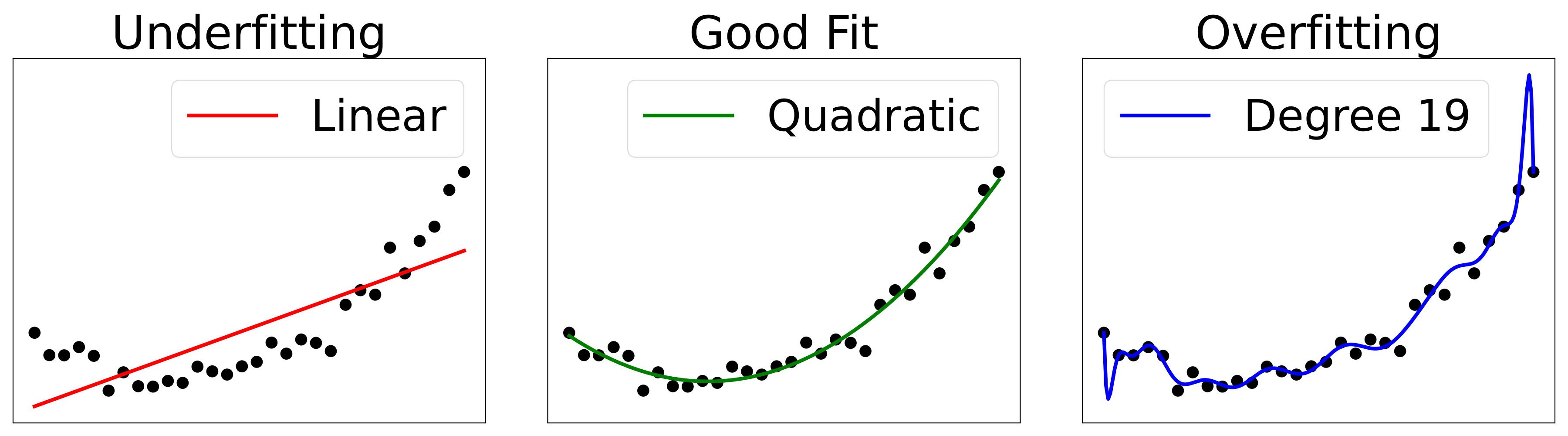
Figure 3: Examples of underfitting and overfitting on a synthetically generated dataset with quadratic structure. Left: A linear fit cannot capture the curvature present in the data. Center: A quadratic fit generalizes well to unseen points and hence does not suffer from a significant amount of either underfitting or overfitting. Right: A polynomial fit of degree 19 suffers from strong overfitting. The solution passes exactly through many points in the dataset, however, the structure has not been correctly extracted, and the performance on unseen data will be poor.

Deep Learning

Deep feedforward networks, also known as MLPs, are the archetype of deep learning models. They are called deep because they have several layers and feedforward because of how the information is progressively fed into the successive layers, flowing towards the output. The term neural is a remnant of the models’ origins in neuroscience, specifically the McCulloch-Pitts neuron [Ref], a simplified model of the biological neuron that can be used as a form of computing element. However, the modern use in deep learning no longer draws these parallels from biology. Finally, these models are called networks because they are typically represented by combining and chaining various neurons together.

A feedforward neural network with three hidden layers is shown in Fig. 4. In our example, input, hidden and output layers have \(n \), \(m \) and \(k \) units, respectively. Moreover, we can see that the network is fully-connected since every neuron of a layer is connected to every neuron in neighboring layers.

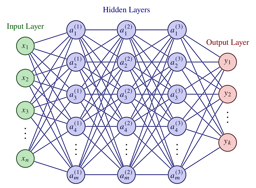
Figure 4: Illustration of a deep feedforward neural network, highlighting its input, output and hidden layers. Adapted from [Ref].

One way to understand neural networks is to consider the limitations of linear models. The obvious problem with linear models is that they are limited to linear functions. In order to extend linear models to approximate nonlinear functions of \(x \), we can apply the linear model not to \(\mathbf{x} \) itself but to a transformed input \(\phi(\mathbf{x}) \), where \(\phi \) is a nonlinear transformation. We can think of this function \(\phi \) as providing a new representation of \(\mathbf{x} \).

So how can this nonlinear transformation \(\phi \) be chosen? We already saw that in classical ML approaches, this is hand-crafted by the engineer. However, here, since deep learning is a type of representation learning, the goal is to learn this transformation \(\phi \). If we assume that this transformation depends on some set of parameters \(\mathbf{w} \), then we can learn what these parameters have to be for a good representation.

So how do we do this? We start from our input say \(\mathbf{x} \). For linear regression, we had:

\[ f(\mathbf{x}; \mathbf{w},b) = \mathbf{x}^\top \mathbf{w} + b\,. \]

The output of this model is a scalar even though the input is a vector. However, if we wanted a multidimensional output, where the linear parameters \(\mathbf{w} \) are different for each dimension, we can organize the parameters in a matrix \(\mathbf{W} \) such that:

\[ \mathbf{h}(\mathbf{x}; \mathbf{W}, \mathbf{b}) = \mathbf{W} \mathbf{x} + \mathbf{b}\,, \]

where now we have a different bias, i.e., additive constant, \((\mathbf{b})_i \) for each output dimension.

Finally, to overcome the defect of linear models, we use a nonlinear function after this affine transformation. This nonlinear function is known as the activation function and can be denoted by \(\mathbf{g} \). Therefore, our model now is as follows:

\[ \mathbf{h}(\mathbf{x}; \mathbf{W}, \mathbf{b}) = \mathbf{g} (\mathbf{W} \mathbf{x} + \mathbf{b} ) \,, \]

where \(\mathbf{g} \) is element-wise. The nonlinear function \(\phi \) now comprises an affine transformation based on the learnable parameters \(\mathbf{W} \) and \(\mathbf{b} \), and a fixed nonlinear function \(\mathbf{g} \). The parameters are adjusted during training, while the form of the activation \(\mathbf{g} \) is chosen beforehand. These operations are also summarized in Fig. 5.

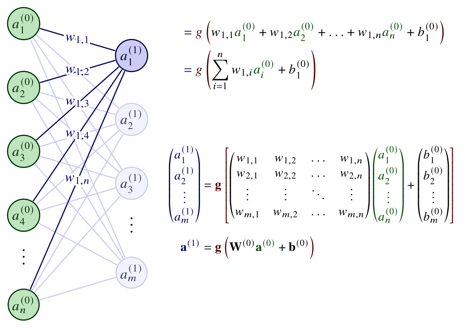
Figure 5: The operations between the input and the first hidden layer. Weights are denoted as \(w \), biases as \(b \), and the activation function as \(g \). The element-wise, vector version of the activation is denoted by \(\mathbf{g} \). Adapted from [Ref].

Various popular activations are plotted in Fig. 6. ReLU has only nonnegative values and is defined as \(\text{ReLU}(x) = \max(0,x) \). It is computationally efficient and mitigates the vanishing gradient problem, making it the default activation for various deep learning architectures. However, it suffers from the so-called “dying ReLU” problem, where neurons can become completely inactive and only output zero for all inputs.

The sigmoid function is defined as \(\sigma (x) = 1/(1+e^{-x}) \), taking values between 0 and 1. While historically important, sigmoid activations are prone to the vanishing gradient problem for large absolute values of the input, which can hamper the training of deep networks, unless intermediate layers designed to avoid this are introduced.

The hyperbolic tangent is defined as \(\tanh (x) = (e^x - e^{-x} )/(e^x + e^{-x}) \) so the function takes values between \(-1 \) and 1. The function is zero-centered which can help with convergence compared to the sigmoid. Nonetheless, it still suffers from vanishing gradients for large inputs.

Finally, the swish function \(\text{swish} (x) = x/(1+e^{-x}) \) [Ref] is an attempt to interpolate between the linear function and the ReLU function. Swish has been shown to outperform ReLU in some deep architectures, especially in deeper models. However, it is computationally more expensive, which can be a serious drawback in resource-constrained settings.

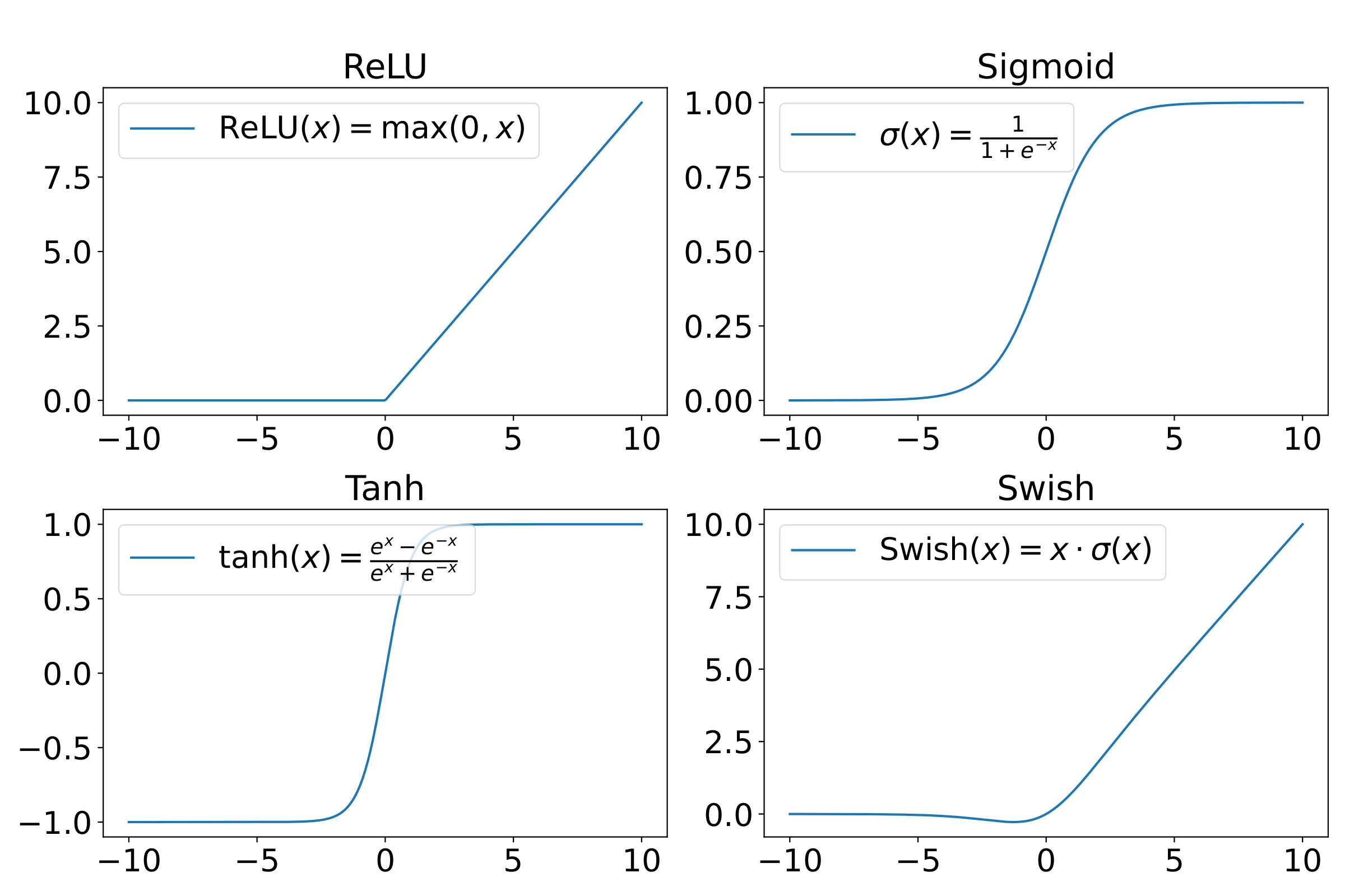
Figure 6: Popular activation functions.

A neural network is nothing more than a chain function of these successive transformations. So, for a \(k \)-layer neural network that returns a scalar, the combined action of the neural network \(f_{\text{NN}} \) on an input \(\mathbf{x} \) is simply:

\[ y = f_{\text{NN}} (\mathbf{x}) = f_k ( \boldsymbol{f}_{k-1} ( \cdots \boldsymbol{f}_2 ( \boldsymbol{f}_1 ( \mathbf{x})))) \,, \]

where \(\boldsymbol{f}_l \), for the layer index \(l = 1,…,k-1 \), are functions with vector output of the form:

\[ \boldsymbol{f}_l (\mathbf{z}) = \mathbf{g_l} (\mathbf{W}_l \mathbf{z} + \mathbf{b}_l) \,, \]

where \(\mathbf{W}_l \) are the weights between layers \(l \) and \(l-1 \), \(\mathbf{g_l} \) and \(\mathbf{b}_l \) are the activation and biases, respectively, of layer \(l \), while \(f_k \) returns a scalar.

The remarkable result of the universal approximation theorem [Ref] states that, under mild assumptions on the activation functions used for the neural network, any continuous function \(f : [0, 1]^n \rightarrow [0, 1] \) can be in fact approximated arbitrarily well by a neural network with as few as one hidden layer and with a finite number of weights. By adding more layers, we are increasing the complexity of the model and hence its capacity to approximate a complex function, as well as to generalize. At the same time, however, we are increasing the computational cost of the algorithm, and therefore, the development of DL models is always a trade-off between these two aspects. By learning the parameters of these models, we essentially can learn how to solve any task, along the representations needed for this specific task.

In order for the learning process to happen, a loss function, similarly to the MSE loss in our linear regression example, is needed. Depending on the problem, a suitable form can be chosen using the MLE method. The weights and biases have then to be chosen such that this function is minimized. This is most frequently done using a form of gradient-based optimization.

Gradient-Based Optimization

Optimization, in general, refers to the minimization or maximization of objective function \(J \), a more general term for what we have been calling the loss function so far. In more general optimization problems—including reinforcement learning and economic modeling—the objective function may take a different form from the loss functions encountered previously, and the goal may instead be to maximize it, such as maximizing a reward signal or economic profit.

For the case of neural networks, we are minimizing the prediction error of the model and this objective function is called a loss function. It is a smooth differentiable function of the parameters \(\boldsymbol{\theta} \) of the model. In addition, even though it has multiple inputs, for the concept of “minimization” to make sense, there must be only one output, i.e., \(J : \mathbb{R}^n \rightarrow \mathbb{R} \). In order to minimize \(J(\boldsymbol{\theta}) \), we need to find the direction, in the \(n \)-dimensional parameter space, that \(J \) decreases the fastest and move in this direction. Since, by the definition of the gradient, \(\nabla_{\boldsymbol{\theta}} J (\boldsymbol{\theta}) \) gives the direction in which \(J \) increases the fastest, we have to update \(\boldsymbol{\theta} \) by going in the opposite direction:

\[ \boldsymbol{\theta} \leftarrow \boldsymbol{\theta} - \alpha \nabla_{\boldsymbol{\theta}} J(\boldsymbol{\theta}) \,, \]

where \(\alpha \) controls the size of the step in this direction and is known as the learning rate. This method proceeds in epochs. An epoch consists of using the entire training dataset to update each parameter. This iterative optimization algorithm is known as gradient descent.

Depending on the size of the dataset, one epoch could be too time consuming for the purposes of developing an ML model. In that case, a family of methods known as Stochastic Gradient Descent (SGD) can be used. For example, instead of using the entire dataset for the parameters updates above, we can sample a mini-batch of data drawn uniformly from the training set. The convergence to a local minimum is thus noisier but significantly faster. At the same time, using this method during training, non-optimal local minima can be avoided.

The process for two learnable parameters is visualized in Fig. 7. Different trajectories can lead to different local minima, potentially resulting in qualitatively distinct outcomes. This problem can be mitigated using optimized versions of these algorithms, with, for example, a variable learning rate. A frequently used example, is the Adam optimizer [Ref]. It combines an adaptive learning rate with momentum, which accumulates a moving average of past gradients to sustain optimization in consistent directions, thereby reducing the risk of stalling in small local minima or flat regions (plateaus) of the loss landscape. In this way, convergence is accelerated and robustness is improved across a wide range of tasks.

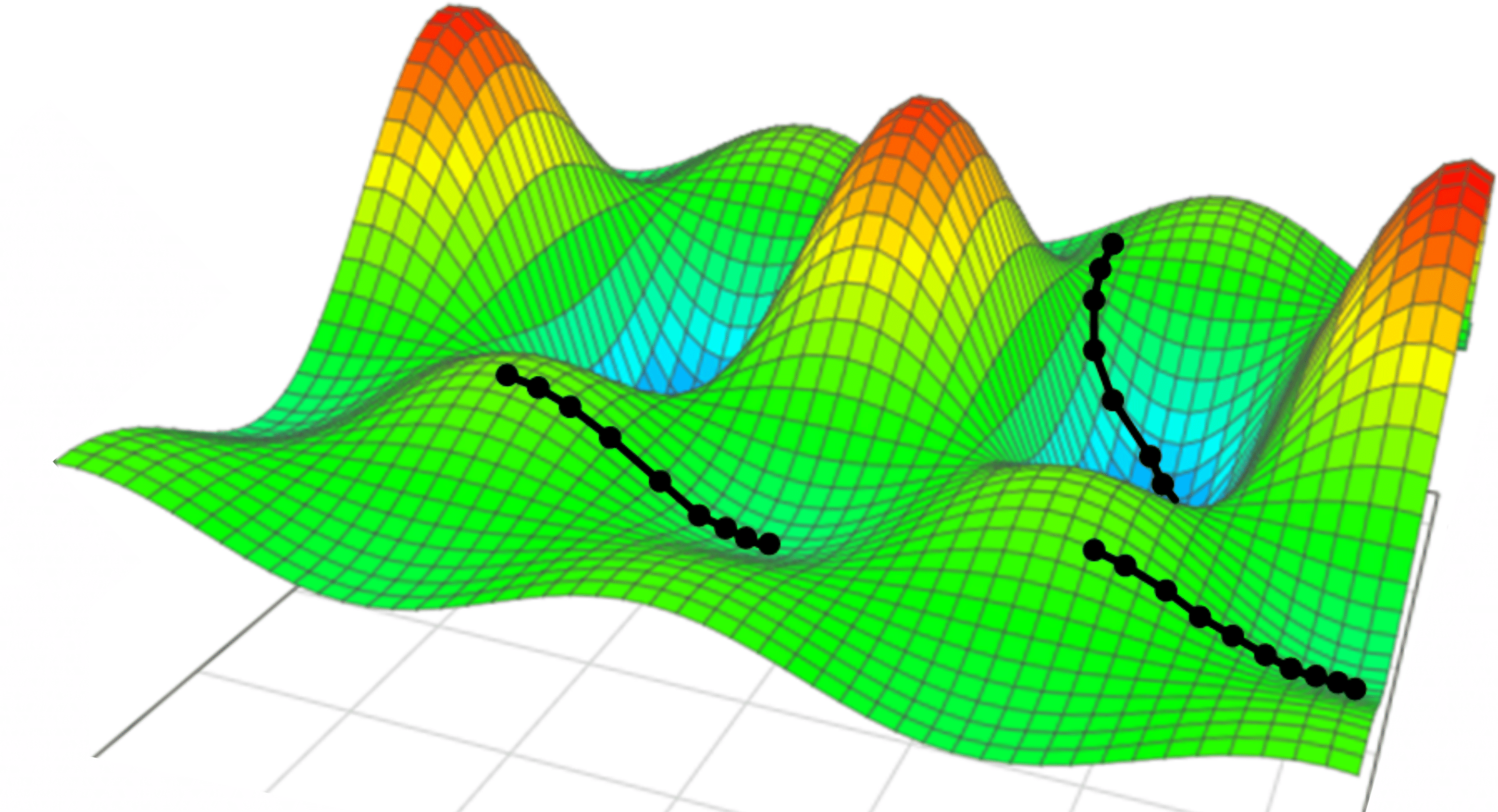
Figure 7: Illustration of gradient descent in a two-dimensional parameter space. Different trajectories may lead to different local minima, and hence may give qualitatively different results. Figure from [Ref].

The next question that arises is the following. Since we said our neural network is essentially a complex nested function of these combinations of nonlinear activations and affine transformations, that means that the loss function is going to have a similar structure. So, how do we know how to update the individual parameters of each layer of the neural network, in order to minimize this objective function?

Backpropagation

When we use a feedforward neural network that accepts an input \(\mathbf{x} \) and produces an output \(\mathbf{y} \), information flows “forward” through the network, as in from left to right in Fig. 4. The input vector \(\mathbf{x} \) provides the initial information that propagates, layer by layer and finally results in \(\mathbf{y} \). This vector \(\mathbf{y} \) is a function of all the weights and biases of all the layers of the neural network, denoted collectively as \(\boldsymbol{\theta} \). This process is known as forward propagation. A scalar cost function \(J(\boldsymbol{\theta}) \) can then be formed using the output \(\mathbf{y} \).

The backpropagation algorithm, is the reverse process where the information from the cost \(J(\boldsymbol{\theta}) \) flows “backward”, i.e., from right to left in Fig. 4, through the network in order to compute the gradients needed for the parameter updates. Essentially, it is an efficient application of the chain rule to neural networks. Backpropagation computes the gradient of a loss function with respect to the parameters of the network for a single input-output example by applying the chain rule layer by layer in reverse order. This backward iteration avoids redundant calculations of intermediate derivatives and is related to dynamic programming, as it reuses intermediate results in order to improve efficiency [Ref].

Strictly speaking, the term backpropagation refers only to the algorithm used for this computation and does not include how the computed gradients are used. The term however, is often used loosely to refer to the entire learning algorithm, including the parameter updates we saw earlier.

Convolutional Neural Networks

Convolutional neural networks are a special kind of deep learning model, especially suited to image data. When the training data are images, the input is high-dimensional. Even for a low resolution image of 256 by 256, the input would have to be of size \(256 \times 256 = 65\,536 \). At this size, using a fully connected feedforward neural network to process the input starts being problematic. In addition, by treating the pixels essentially as a vector, we lose information about the “local structure” of the image. Apart from the value of the pixel itself, there is a significant amount of information in the placement of the pixels relative to each other. Going back to our earlier example, even by changing the value of the pixel colors, one could still understand whether a photo depicts a grass field or not. The information of the texture of the grass is somehow encoded in how the relative values of the pixels are arranged together to form the edges that correspond to the grass blades, and the patterns in general, which together convey the texture and structure typical of a grass field.

In order to capture this local structure of the image, the idea is to instead of flattening the input into a vector, to process it in its original, matrix-like, form. To make this easier, we can split the image into small square patches, of equal size. Each patch can then be processed to extract meaningful local features. In practice, this is done using shared filters, also known as kernels, that learn to detect patterns relevant to the task. How can this really be done?

In order to preserve the local structure, we organize the learnable parameters of the model in a matrix \(\mathbf{F} \), for “filter”, of size equal to the size of the patches. We then perform the convolution of the filter matrix \(\mathbf{F} \), across the original image using a moving window approach, as illustrated in Fig. 8. The pixels of the patch are multiplied element-wise into a scalar, and then the bias is added. The output of this operation is sometimes referred to as the feature map. Like before, a nonlinearity is applied to the output, typically the ReLU activation. The learnable parameters of this algorithm are the values of the matrix “filter” as well as the value of the “bias”.

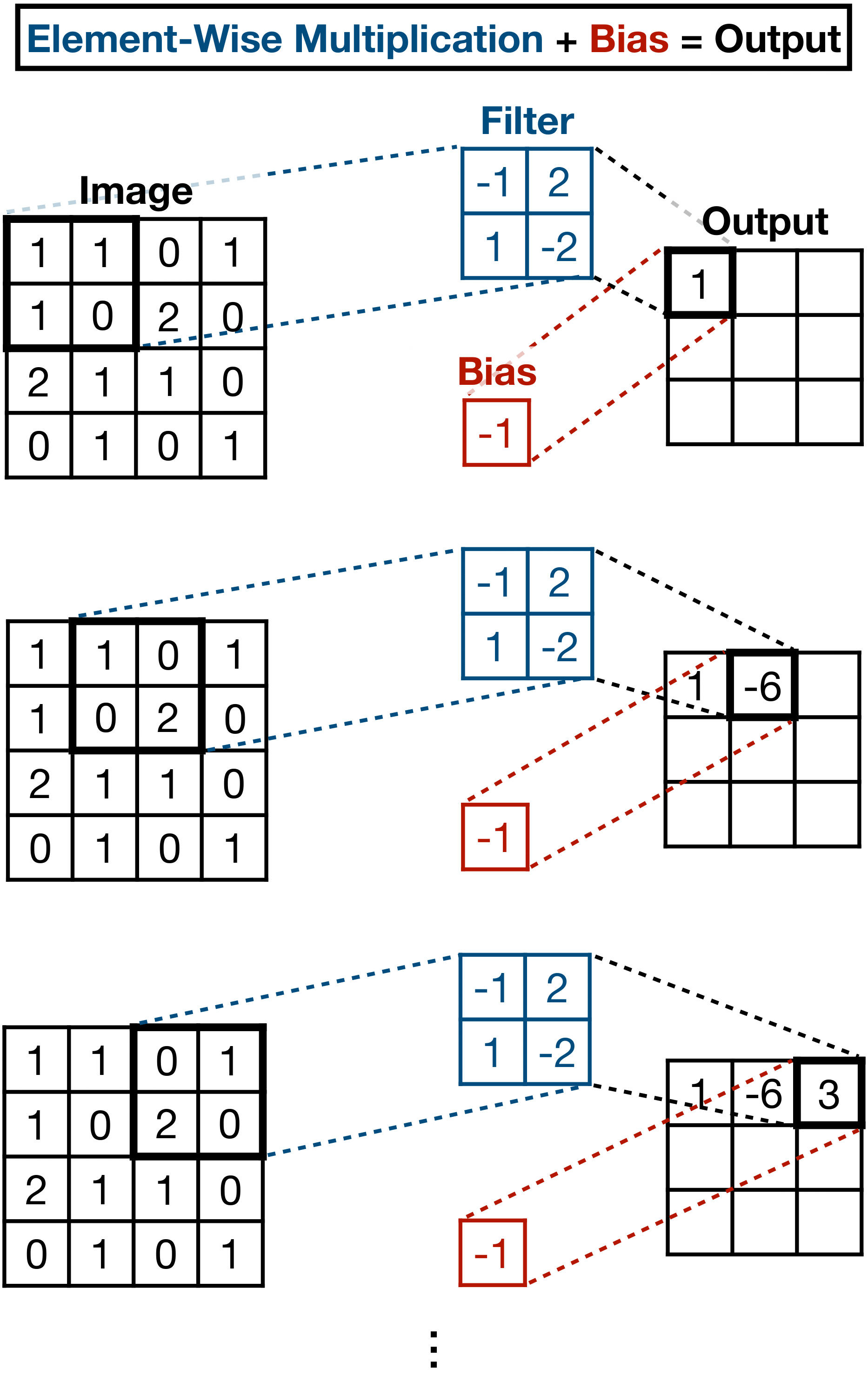
Figure 8: Illustration of the process of convolving a filter across an image using a sliding window approach. Inspired by [Ref].

This operation is performed for a number \(k \) of filters, in order to extract various features in the image, and each filter’s parameters are completely independent. The output for each filter is different, and hence the operation of this convolutional layer results in a collection of \(k \) feature maps. This collection can be thought of as a higher-dimensional tensor and is called a volume. For color images, the input is actually also a volume, since the image is usually represented by three channels: R (red), G (green), and B (blue), where each channel is a monochrome picture.

In a convolutional layer with a multi-channel input volume, the operation is similar to the single-channel case. The convolution of a patch from a multi-channel volume is equal to the sum of the convolutions of the corresponding patches from each individual channel.

By applying various convolutional layers in sequence, the model can learn hierarchical representations of data, starting from low-level representations such as edges in images, all the way to high-level features such as faces and objects.

Another operation frequently used in CNNs is pooling. It works in a similar way to the convolution, as a filter is applied using a sliding window approach. However, instead of applying a trainable filter, a fixed operation is applied: commonly max pooling (which selects the maximum value) or average pooling (which computes the mean value) within each window. Pooling is used to reduce the spatial dimensions of feature maps, helping to retain the most significant features from the input. This subsampling process lowers the number of parameters, decreases computation time, and helps prevent overfitting, ultimately improving model performance.

A famous and illustrative example of the CNN architecture is shown in Fig. 9. The LeNet-5 architecture [Ref], designed for digits recognition, is split into two modules: the feature extraction module and the trainable classifier module. For the former, a convolutional layer is combined with a subsampling layer twice, C1-S2 and C3-S4, and then layer C5 creates 120 feature maps of size \(1\times 1 \). These feature maps are then “flattened” into a 1-dimensional vector of size 120. For the classification part, this vector is then fed into the feedforward fully connected layers.

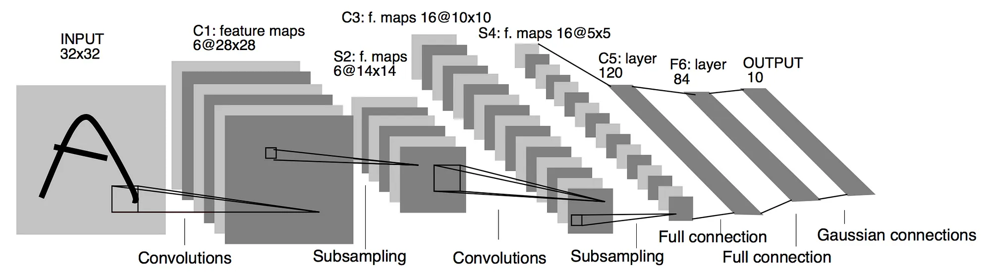
Figure 9: The architecture of LeNet-5, a convolutional neural network for digits recognition, as depicted in the original paper [Ref]. The feature extraction module is illustrated using convolution and pooling operations. The classification is performed in the fully connected layers. The input is images of size \(32 \times 32 \). Layer C1 has 6 feature maps of size \(28 \times 28 \), while layer C3 has 16 feature maps of size \(10\times10 \). After subsampling, layers S2 and S4 reduce the size of the maps by one half. The output is then fed into the fully connected network of layers with 120 and 84 units. Finally, the output of the network is a vector of dimension 10.

Graph Neural Networks

What happens when the data that we have are not structured in the traditional tabular manner, such as vectors in the case of series, or matrices in the case of images? Furthermore, what happens when our data possess an inherent network structure which we would like to take into account, or even learn about directly?

Networks are ubiquitous—and so are graphs. In many real-world scenarios, it is beneficial to think of data points not in isolation but as part of a web of complex connections: people connected through social interactions, proteins by biochemical interactions, or web pages by hyperlinks. Capturing and using this connectivity is crucial for understanding the underlying relationships and dynamics [Ref].

Similarly to images being processed by CNNs, we would like to have an algorithm that can have these complex network structures as input. These structures are known as graphs. In general, a graph is a pair \(G = (V, E) \), where \(V \) is a finite set of vertices (or nodes), and \(E \) is the set of connections (known as edges) between these nodes. Graphs can be further classified into directed and undirected. The former means that the edges have a certain direction, for example, we can go from node 5 to 6, but not the other way around, as illustrated in Fig. 10. The latter means that the connections are only symmetrical and mutual, as illustrated in Fig. 11. In addition, in Fig. 11, we can see that the graph comprises two so-called connected components, i.e., maximally connected subgraphs which are disconnected with each other.

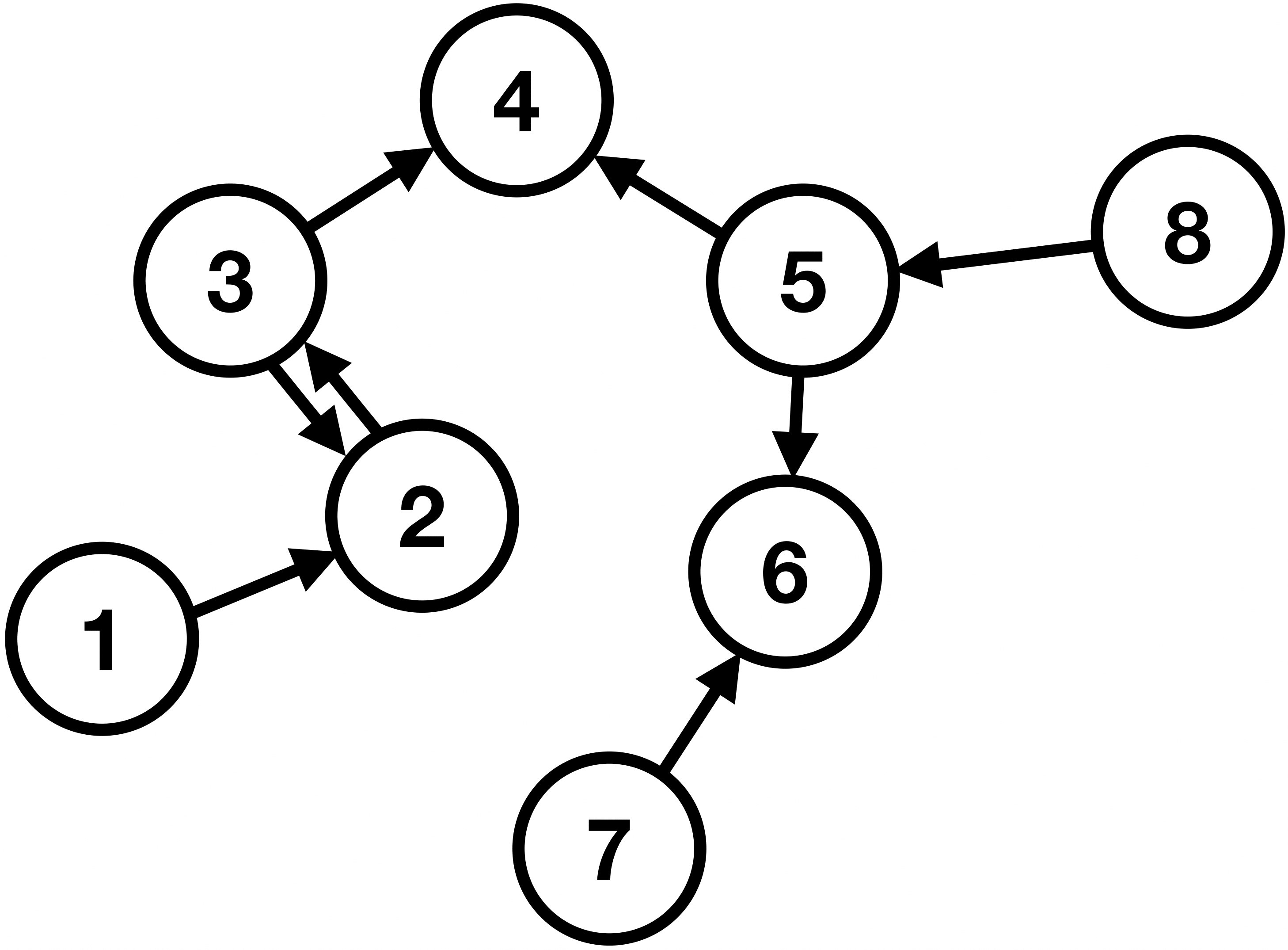
Figure 10: A directed graph with eight vertices and seven edges.

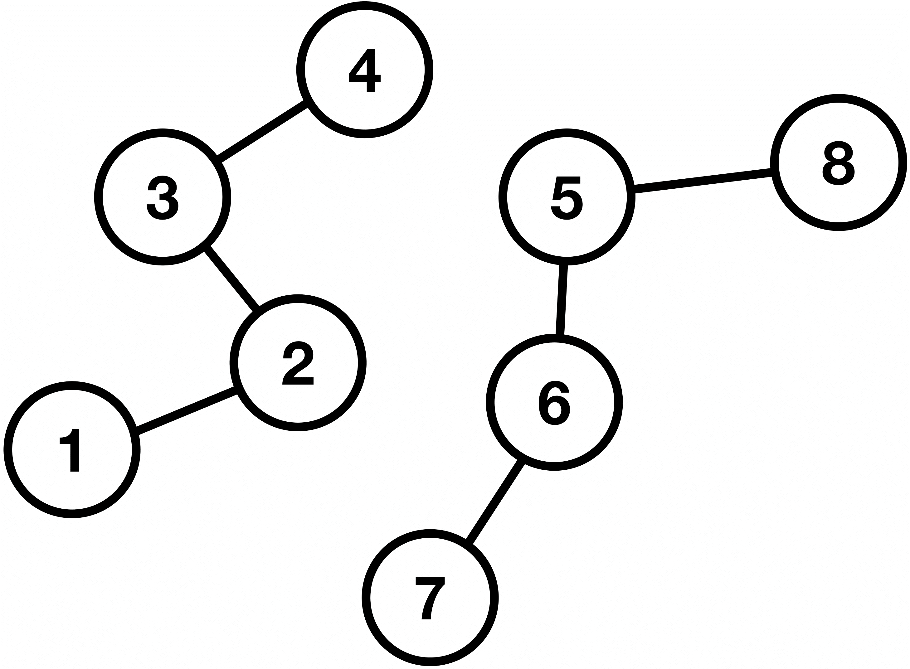
Figure 11: An undirected graph with eight vertices and seven edges, and two connected components.

Graphs can be represented in various ways. A frequently used representation is the so-called adjacency matrix. The elements of the adjacency matrix \(\mathbf{A} \) are given simply by \( \mathbf{A}_ {ij} = 1 \), if there is a link from node \(i \) to node \(j \), and \( \mathbf{A}_ {ij} = 0 \), otherwise.

The adjacency matrix \(\mathbf{A} \) is therefore symmetric for undirected graphs but not necessarily symmetric for directed ones. Furthermore, the edges themselves, may possess some value based on some characteristic, instead of simply 0 and 1. In this case, the graph is called weighted. Finally, the information associated with the nodes is referred to as node features, while the information associated with the edges is known as edge features.

The question now is the following: How do we take advantage of the relational structure of graphs, in order to achieve better predictions? Drawing inspiration from CNNs, where we wanted to capture the local structure of the pixels in the images, we will try to do something similar. The idea is to do a series of “convolutions”, similar to the ones for images, but this time suited for data with a network structure.

Node Embeddings

Similarly to deep learning, we wanted to avoid hand-designing the representations of the problem, and we tried to learn them, in a process that we called representation learning. In the same vein, we will use the same method for our graphs. We will learn node representations, which we will call node embeddings, that will contain information about any node and its connections to neighboring nodes. In this mapping, that can be learned using a neural network, similar nodes in the network are embedded close to each other.

Message Passing

In order to capture and encode inside the node embeddings the connectivity of the network, for each node in the graph, the process is as follows [Ref].

1. The embeddings of neighboring nodes are aggregated using a permutation invariant function. This is justified because a permutation of the graph nodes should not give a different result. Examples of these aggregating functions include the max, sum or average functions. This process is referred to as the aggregation of the messages received from the immediate neighbors.
2. This aggregated information is then passed through a neural network.
3. Finally, the node embedding of the target node is updated based on the aggregated messages from its neighbors. This iterative process of updating the node representations by exchanging information between neighbors is known as message passing.

In this way, after each message passing step, the receptive field of the GNN increases by one hop. Hop, here, refers to a traversal from one node of a graph to a neighboring node via a connecting edge. The process is summarized in Fig. 12.

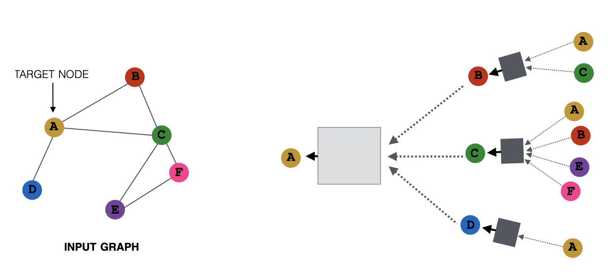
Figure 12: Illustration of the process of message passing. Every node defines its own computation graph based on its neighborhood. Left: The input graph and the target node based on which the series of computations is defined. Right: The message passing steps for two hops away from the target node. Gray rectangles represent neural networks. Figure from [Ref].

For a graph \(G = (V,E) \), the message passing layer can also be expressed as:

\[ \mathbf{h}_ u = \phi \left( \mathbf{x}_ u, \bigoplus_ {v \in \text{Adj}[u]} \psi (\mathbf{x}_ u, \mathbf{x}_ v,\mathbf{e}_ {uv}) \right) \,, \]

where \(\phi \) and \(\psi \) are differentiable functions representing neural networks, \(\text{Adj}[u] \) is the immediate neighborhood of node \(u \in V \), \(\mathbf{x}_ u \) represents the node features of node \(u \in V \), and \(\mathbf{e}_ {uv} \) represents the edge features of edge \((u,v) \in E \). Finally, \(\bigoplus \) is a permutation invariant aggregation operator (e.g., element-wise sum, mean) accepting an arbitrary number of inputs. Functions \(\phi \) and \(\psi \) are referred to as the update and message functions, respectively.

Other “flavors” of this message passing process have been developed, such as the famous graph convolution networks [Ref] and interaction networks [Ref].

Having presented these ML models, we now move on to an important technique used in the field of ML/DL: quantization.

Quantization

Quantization, in signal processing in general, is the process of mapping a set of values from a continuous set to a finite set. Examples of this include rounding and truncation. In this form, quantization is involved to some extent in nearly all digital signal processing, because the continuous analog signal of any quantity has to be digitized, to discrete values.

In the context of ML/DL [Ref], quantization refers to a process of reducing the size of the models, by representing their weights and activations using numbers with less bits than standard floating-point systems, where 32 or 64 bits are typical. In this way, the computational and memory costs of inference can be reduced significantly. On the one hand the required memory is reduced because simply the space required by each weight is reduced. On the other hand, the operations happen between low-precision data types and hence are considerably less computationally expensive.

As a simple example, let’s consider a symmetric quantization scheme, from 32-bit float to 8-bit integer precision. With 8 bits, only \(2^8 = 256 \) numbers can be represented, while using 32-bit floats, a wide range of values is possible. Let’s consider a float \(x \in [-\alpha,\alpha] \), where \(\alpha \) is a real number with \(\alpha>0 \). How do we best project this symmetric interval \([-\alpha,\alpha] \) of floats onto the space of 8-bit integers? We can write the following quantization scheme:

\[ x = S \times x_q \,, \]

where \(x_q \) is the quantized representation of float \(x \), and float \(S \) is the scale quantization parameter. The quantized value can then be calculated as follows:

\[ x_q = \text{round}(x/S) \,. \]

Finally, any float values outside interval \([-\alpha,\alpha] \) are clipped, so for any float \(x \):

\[ x_q = \text{clip}(\text{round}(x/S), -\alpha_q, \alpha_q) \,, \]

where \(\alpha_q = \text{round}(\alpha/S) \), and \(\text{clip}(x, x_{\text{min}}, x_{\text{max}}) \) denotes the clamp (or clipping) function between \(x_{\text{min}} \) and \(x_{\text{max}} \).

Calibration and Quantization Types

Calibration is the process during which the ideal values for the quantization parameters, the scale \(S \) in our example, are chosen based on the distribution of the input values. For example, as shown in Fig. 13, based on the range of the input values, the interval limits \([-\alpha,\alpha] \) are chosen, and the value of \(S \) is chosen such that \(\alpha \) is mapped to the highest value the quantized type can take. For the values shown, and according to the equations above, the scale will have to be \(S = 10.8 / 127 \). Due to the interval being symmetric, from the 256 available values in INT8, we effectively only have half the numbers to represent positive values, while the rest are reserved for the zero point and the negative values.

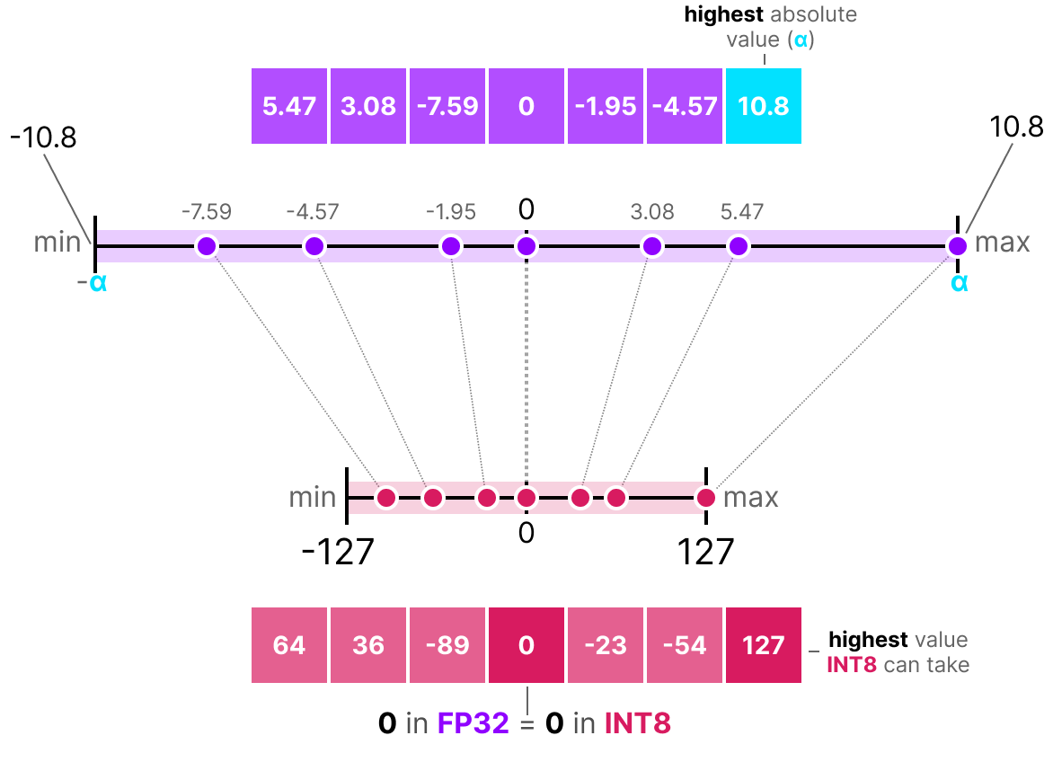
Figure 13: Illustration of the process of symmetric quantization. The scale is chosen to best fit the input values to be quantized. Figure from [Ref].

For the case of neural networks, the input values of the quantization are the weights and the activations of the model. For weights, the process is quite easy since the actual range can be easily calculated at the time of quantization. For activations, however, things are a bit more complicated, and the approaches are different depending on the type of quantization pursued:

• Post-Training Quantization (PTQ): The quantization of the weights and activations is performed after the training of the model in full precision.
• Quantization-Aware Training (QAT): The quantization is performed during the training process.

Depending on the type of quantization, a different method for the calibration of the activations is used [Ref]:

• Static PTQ: At the time of quantization, a representative sample of the data is passed through the model and the activation values are recorded, using “observers” placed at the activations. After several forward passes, the ranges of the computations can be deduced using some calibration technique.
• Dynamic PTQ: For each activation, the range is computed at runtime. However, this can prove slow and even not an option on several types of hardware.
• QAT: The ranges of computations are computed during training. “Fake quantize” operators simulate the effects of quantization during training, enabling the model to adjust and become robust to the errors introduced by the quantization process.

Conclusion

In this article, I presented a brief history of machine learning, and sketched, from the ground up, the inner workings of graph neural networks. Quantization was also introduced.

This article is one of the chapters of my PhD thesis titled: “Real-Time Analysis of Unstructured Data with Machine Learning on Heterogeneous Architectures”. The full text can be found here: PhD Thesis. In the main results part of this work, GNNs were used to perform the task of track reconstruction, in the context of the Large Hadron Collider at CERN.