Modeling Earthquake Clustering: Poisson vs. Hawkes Processes

How do we model the timing of rare events? Earthquakes, disease outbreaks, or neuron spikes all occur as sequences of events in time. The simplest assumption is that these events are independent and random, following a homogeneous Poisson process. But in reality, many event sequences exhibit clustering: one event increases the probability of future events.

Earthquakes are a perfect example. When a large earthquake occurs, it triggers a cascade of aftershocks. These aftershocks are not independent—they are directly caused by the stress redistribution from the main shock. This phenomenon is called self-excitation.

In this post, we explore temporal point processes and compare two models:

1. Homogeneous Poisson Process – independent events at constant rate
2. Hawkes Self-Exciting Process – events that cluster due to self-triggering

We apply both models to real earthquake data from Greece (2016–2026) and demonstrate why the Hawkes process provides a dramatically better explanation for earthquake clustering.

The code can be found on Github at the end of this post.

Background: Temporal Point Processes

A temporal point process is a stochastic process that generates a sequence of events in time. We represent this as a collection of event times:

\[ {t_1, t_2, \ldots, t_n} \]

The fundamental quantity that characterizes a point process is the intensity function \(\lambda(t)\), which represents the instantaneous rate of events at time \(t\), conditioned on the history of past events.

For a small time interval \(dt\):

\[ \mathbb{P}(\text{event in } [t, t+dt) \mid \mathcal{H}_t) = \lambda(t \mid \mathcal{H}_t) \, dt \]

where \(\mathcal{H}_t\) is the history of events up to time \(t\).

General Likelihood of a Point Process

Both models below are fit by maximizing the same general log-likelihood:

\[ \log \mathcal{L} = \sum_{i=1}^{n} \log \lambda(t_i) - \int_0^T \lambda(t) \, dt \]

This can be derived directly from the intensity definition above. Partition \([0, T]\) into \(N\) tiny bins of width \(\Delta t = T/N\). By definition, the probability of an event occurring in the bin \([t, t + \Delta t)\) is \(\approx \lambda(t) \Delta t\), so the probability of no event in that bin is \(\approx 1 - \lambda(t)\Delta t\).

The observed data is: an event in each of the \(n\) bins containing \(t_1, \ldots, t_n\), and no event in every other bin. Since bins are (approximately) independent given the history, the likelihood of this exact realization is a product over all bins:

\[ \mathcal{L} \approx \underbrace{\left[\prod_{i=1}^{n} \lambda(t_i) \Delta t\right]}_{\text{bins with an event}} \times \underbrace{\prod_{\text{empty bins}} \big(1 - \lambda(t)\Delta t\big)}_{\text{bins with no event}} \]

Dropping the constant factor \(\Delta t^n\) (it doesn’t depend on the parameters, so it doesn’t affect maximization) and using \(1 - x \approx e^{-x}\) for small \(x\), the empty-bin product becomes a Riemann sum in the exponent:

\[ \prod_{\text{empty bins}} \big(1 - \lambda(t)\Delta t\big) \approx \exp\left(-\sum_{\text{empty bins}} \lambda(t)\Delta t\right) \xrightarrow{\Delta t \to 0} \exp\left(-\int_0^T \lambda(t) \, dt\right) \]

Putting the two pieces together gives \(\mathcal{L} = \left[\prod_{i=1}^n \lambda(t_i)\right] \exp\left(-\int_0^T \lambda(t)\,dt\right)\), and taking logs recovers the formula above. Every model in this post — Poisson, Hawkes, Marked Hawkes, ETAS — is just a different choice of \(\lambda(t)\) plugged into this same expression.

The Poisson Process

The simplest model is the homogeneous Poisson process, where the intensity is constant:

\[ \lambda(t) = \lambda \]

This means:

• Events occur independently
• The rate is time-invariant
• Inter-arrival times follow an exponential distribution

Likelihood for Poisson

Given observed event times \({t_1, \ldots, t_n}\) up to time \(T\), the log-likelihood is:

\[ \log \mathcal{L}(\lambda) = n \log \lambda - \lambda T \]

This follows from the general log-likelihood of a temporal point process,

\[ \log \mathcal{L} = \sum_{i=1}^{n} \log \lambda(t_i) - \int_0^T \lambda(t) \, dt, \]

by plugging in a constant intensity \(\lambda(t) = \lambda\): the sum collapses to \(n \log \lambda\) since every term is identical, and the integral becomes \(\lambda T\) since \(\lambda\) doesn’t depend on \(t\).

The maximum likelihood estimator is simply:

\[ \hat{\lambda} = \frac{n}{T} \]

which follows from setting \(\partial \log \mathcal{L} / \partial \lambda = n/\lambda - T\) to zero.

Why Poisson Fails for Earthquakes

The Poisson model assumes that knowing past earthquakes tells us nothing about future earthquakes. But this contradicts seismological reality:

• Main shocks are followed by clusters of aftershocks
• Triggering happens over hours, days, and weeks
• Magnitude correlates with the intensity and duration of aftershock sequences

For Greece (2016–2026), fitting a Poisson model to the full USGS catalogue gives \(\hat{\lambda} \approx 0.638\) events/day, which predicts that earthquake times should look “random.” But the actual data shows clear clustering, with far more very short waiting times than a Poisson model would predict.

The Hawkes Self-Exciting Process

The Hawkes process is a point process where the intensity depends on the entire history of past events:

\[ \lambda(t) = \mu + \sum_{t_i < t} \alpha e^{-\beta(t - t_i)} \]

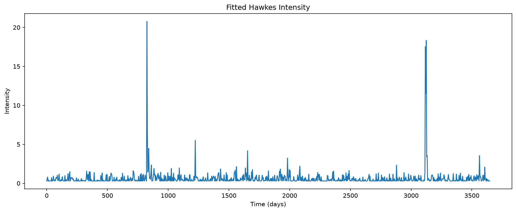
Figure 1: Hawkes intensity function. Each event (vertical line) causes an instantaneous jump in intensity, followed by exponential decay. Notice the clustering: events trigger more events.

Interpretation

• \(\mu\): background intensity – spontaneous seismic activity
• \(\alpha\): triggering strength – how much each earthquake increases future risk
• \(\beta\): decay rate – how quickly aftershock risk diminishes
• \(e^{-\beta(t - t_i)}\): kernel – exponential decay from each past event

Key property: When an earthquake occurs at time \(t_i\), the intensity jumps up by \(\alpha\) and then exponentially decays back to \(\mu\) with timescale \(\beta^{-1}\).

This is called self-excitation: the process triggers itself.

Connection to Seismology

In seismology, the aftershock rate follows Omori’s law:

\[ n(t) = \frac{K}{(t + c)^p} \]

The Hawkes exponential kernel is a related but simpler approximation that leads to tractable inference.

Likelihood for Hawkes

The log-likelihood for observed events \({t_1, \ldots, t_n}\) over interval \([0, T]\) is:

\[ \log \mathcal{L}(\mu, \alpha, \beta) = \sum_{i=1}^{n} \log \lambda(t_i^-) - \int_0^T \lambda(t) \, dt \]

where \(\lambda(t^-)\) is the intensity just before event \(t_i\) occurs (excluding the event itself).

The intensity at event time \(t_i\) is:

\[ \lambda(t_i^-) = \mu + \sum_{j < i} \alpha e^{-\beta(t_i - t_j)} \]

The integral can be computed analytically by splitting the sum and integrating each exponential kernel term-by-term:

\[ \int_0^T \lambda(t) \, dt = \mu T + \sum_{j=1}^{n} \int_{t_j}^{T} \alpha e^{-\beta(t - t_j)} \, dt = \mu T + \sum_{j=1}^{n} \frac{\alpha}{\beta} \left(1 - e^{-\beta(T - t_j)}\right) \]

using \(\int_{t_j}^{T} e^{-\beta(t - t_j)} \, dt = \frac{1}{\beta}\left(1 - e^{-\beta(T - t_j)}\right)\), the standard integral of a decaying exponential.

Implementation

Here is the core implementation in Python:

import numpy as np

def intensity(t, history, mu, alpha, beta):
    """
    Compute Hawkes intensity at time t.
    
    Parameters:
    - t: current time
    - history: array of past event times
    - mu, alpha, beta: Hawkes parameters
    """
    if len(history) == 0:
        return mu
    
    return (
        mu + 
        np.sum(alpha * np.exp(-beta * (t - history)))
    )


def hawkes_log_likelihood(params, times):
    """
    Compute Hawkes log-likelihood for observed event times.
    
    Parameters:
    - params: (mu, alpha, beta)
    - times: sorted array of event times
    
    Returns:
    - log-likelihood (or -inf if parameters invalid)
    """
    mu, alpha, beta = params
    
    # Parameter constraints
    if mu <= 0 or alpha < 0 or beta <= 0:
        return -np.inf
    
    # Event contribution: sum of log intensities
    log_sum = 0
    for i, t in enumerate(times):
        history = times[:i]
        lam = intensity(t, history, mu, alpha, beta)
        log_sum += np.log(lam)
    
    # Integral contribution
    T = times[-1]
    integral = (
        mu * T + 
        np.sum(
            alpha / beta * (1 - np.exp(-beta * (T - times)))
        )
    )
    
    return log_sum - integral

Maximum Likelihood Estimation

To estimate parameters, we maximize the log-likelihood using numerical optimization:

from scipy.optimize import minimize

def fit_hawkes(times):
    """Fit Hawkes parameters using maximum likelihood."""
    
    # Initial guess
    mu0 = len(times) / (times[-1] - times[0])
    alpha0 = 0.5 * mu0
    beta0 = 1.0
    
    # Optimize
    result = minimize(
        lambda p: -hawkes_log_likelihood(p, times),
        x0=[mu0, alpha0, beta0],
        method='Nelder-Mead'
    )
    
    return result.x

Real Data: Greece Earthquakes 2016–2026

We use the USGS Earthquake Catalog for Greece over 10 years (2016–2026). The dataset contains:

• 2,325 earthquakes recorded between 23 July 2016 and 18 July 2026 (≈3,647 days)
• Magnitude: ranges from 2.5 to 7.0, mean \(\approx 4.38\)
• Time: ISO 8601 format (UTC)
• Location: latitude, longitude, depth

Fitting Results

Fitting both models to the Greece data gives the following parameter estimates:

Poisson Process:

• \(\hat{\lambda} \approx 0.638\) events/day (\(\approx 233\) events/year)
• Log-likelihood: \(\log \mathcal{L}_{\text{Poisson}} \approx -3371\)

Hawkes Process:

• \(\hat{\mu} \approx 0.296\) events/day (background)
• \(\hat{\alpha} \approx 0.908\) (strong triggering)
• \(\hat{\beta} \approx 1.695\) /day (aftershocks decay with a half-life \(\approx 0.41\) days, under 10 hours)
• Branching ratio \(n = \alpha/\beta \approx 0.536\): about 54% of earthquakes are themselves triggered by an earlier one
• Log-likelihood: \(\log \mathcal{L}_{\text{Hawkes}} \approx -1816\)

Simulating Each Model

To visually check each fit against the real catalogue, we generate a synthetic earthquake sequence from each model using its fitted parameters:

• Poisson: draw i.i.d. exponential waiting times with rate \(\hat\lambda\), and accumulate them until reaching the end of the observation window.
• Hawkes: use Ogata’s thinning algorithm — propose candidate times from an upper-bound intensity, then accept or reject each proposal based on the true, history-dependent intensity at that time. Accepted events feed back into the intensity, so clustering emerges naturally from the accepted sequence.

Poisson simulation

Simulating the Poisson model with this rate and comparing it to the real catalogue:

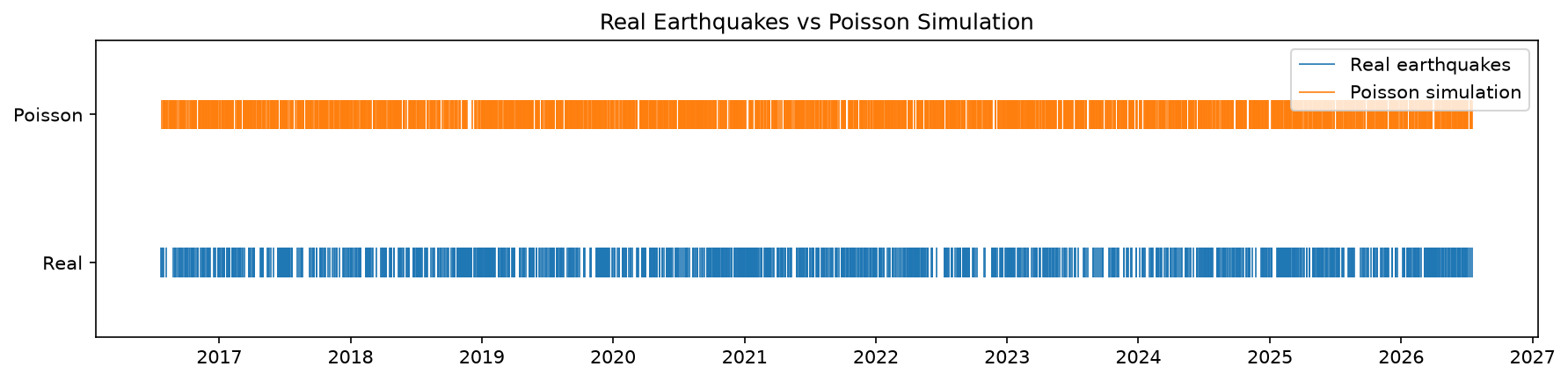
Figure 2: Real Greece earthquakes (bottom) vs. a simulated Poisson process with the fitted rate \(\hat\lambda \approx 0.638\)/day (top), over the same 2016–2026 window. The Poisson simulation spreads events roughly uniformly in time, while the real catalogue shows visible bursts and gaps.

The timeline hints at a mismatch, but the waiting-time distribution makes it precise. A Poisson process is memoryless: the gap until the next event is exponentially distributed regardless of how recently the last one occurred. That forces a smooth, single-peaked decay in waiting times. The real catalogue instead front-loads far more probability onto very short gaps — the direct footprint of aftershocks arriving within hours of a mainshock — which a constant-rate model has no mechanism to produce:

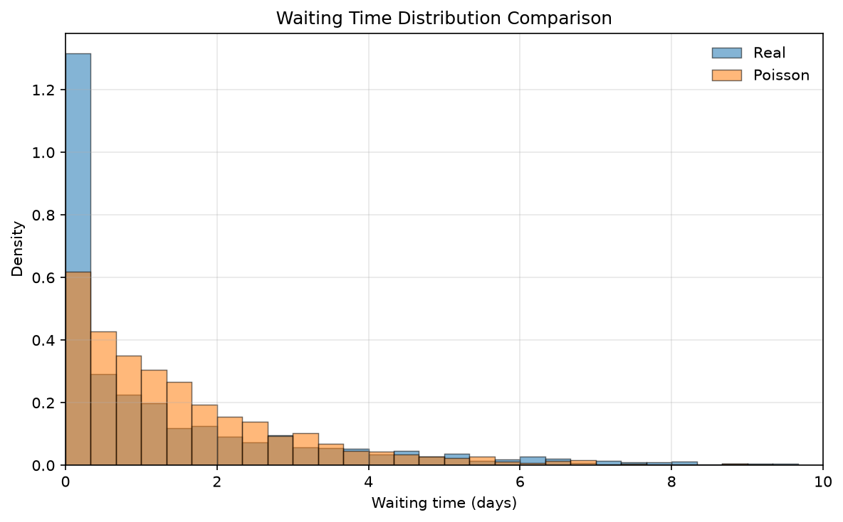
Figure 3: Distribution of waiting times (days between consecutive earthquakes): real data vs. the fitted Poisson process. The real data has far more very short waiting times than Poisson predicts — a direct signature of clustering that a constant-rate model cannot capture.

Hawkes simulation

Using the fitted \(\mu, \alpha, \beta\) and Ogata’s thinning algorithm, we simulate a synthetic Hawkes sequence. It produces 2,441 synthetic events — close to the 2,325 real earthquakes — and the resulting sequence visually resembles the real data:

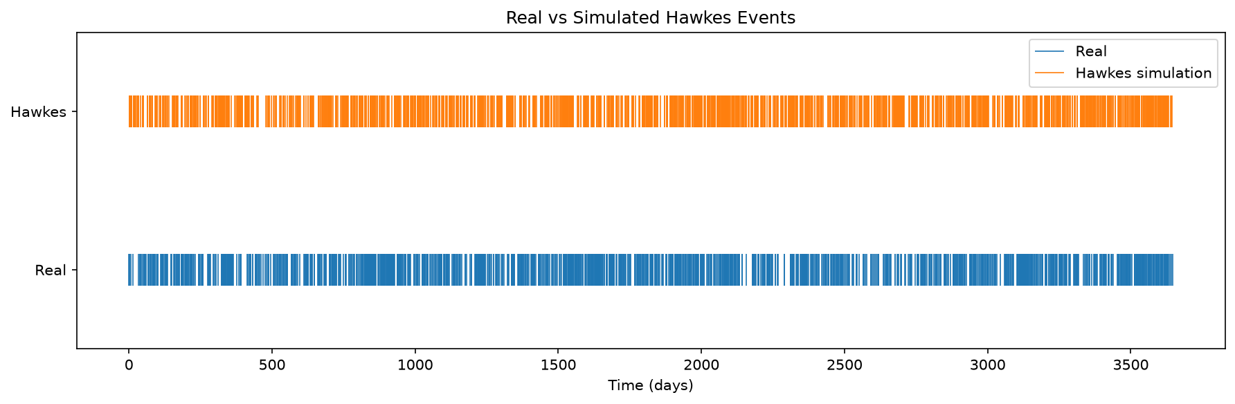
Figure 4: Real Greece earthquakes (bottom) vs. a simulated Hawkes process with the fitted parameters (top). Both series show similar bursty structure — the Hawkes simulation reproduces the clustering visible in the real catalogue far better than a Poisson simulation would.

• Clustering: bursts of aftershocks following mainshocks
• Duration: clusters persist for weeks
• Rate variation: quiet periods interrupted by active sequences

Poisson simulations, by contrast, show uniform random spacing with no clusters. The same gain shows up in the waiting-time distribution: because the Hawkes intensity jumps after every event and decays over a roughly 10-hour half-life, the simulated waiting times closely track the real data’s excess of very short gaps — the exact feature the Poisson fit above missed:

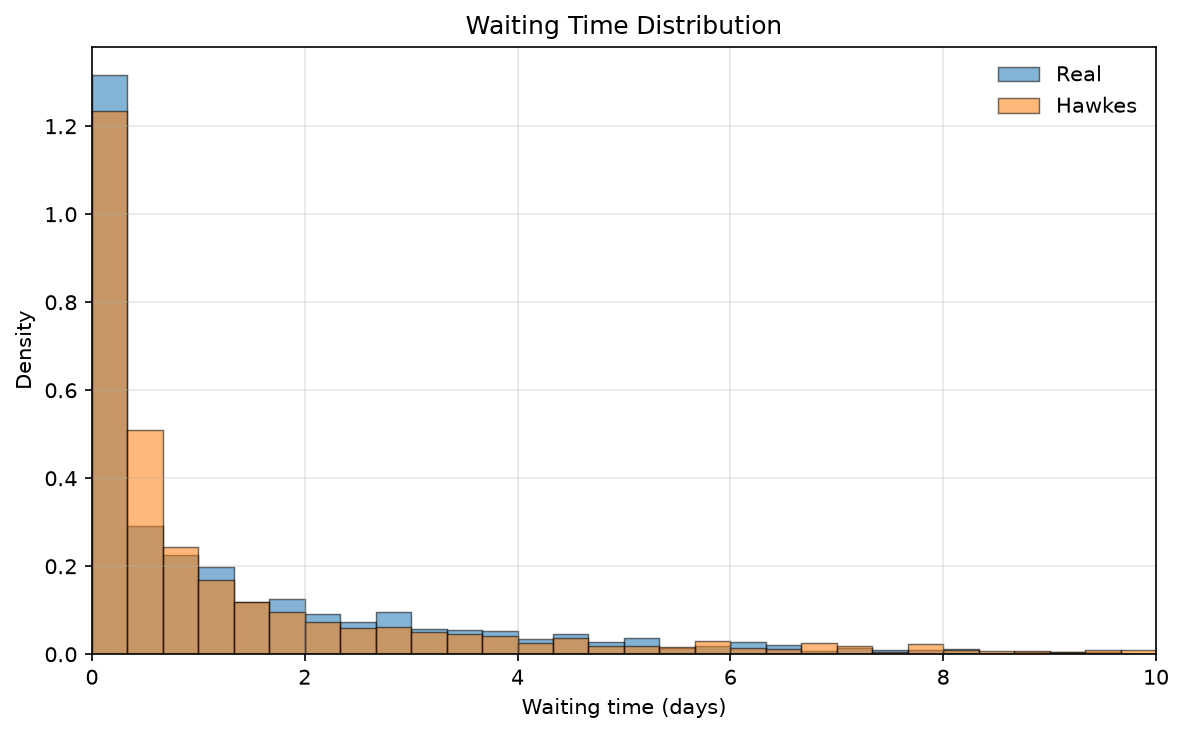
Figure 5: Same waiting-time comparison, real data vs. the fitted Hawkes process. Unlike the Poisson fit, the Hawkes distribution closely tracks the real data across the full range of waiting times, including the excess of very short gaps.

Likelihood Ratio Test:

A higher log-likelihood for Hawkes isn’t proof by itself — a model with more parameters can never fit worse than a model it contains as a special case, so some improvement is guaranteed even if the extra parameters were fitting pure noise. Setting \(\alpha = 0\) collapses the Hawkes intensity \(\lambda(t) = \mu + \sum_{t_i < t} \alpha e^{-\beta(t-t_i)}\) back to \(\lambda(t) = \mu\), i.e. exactly the Poisson model — so Poisson is a nested restriction of Hawkes, which is precisely the condition needed for a likelihood ratio test to apply.

Under the null hypothesis \(H_0: \alpha = 0\) (earthquakes really are Poisson), the test statistic

\[ -2 \log \frac{\mathcal{L}_{\text{Poisson}}}{\mathcal{L}_{\text{Hawkes}}} \approx 3110 \]

asymptotically follows a \(\chi^2_2\) distribution (2 degrees of freedom, matching the 2 extra parameters \(\alpha, \beta\)). With 2 extra parameters (\(\alpha, \beta\) versus just \(\lambda\)), this vastly exceeds the \(\chi^2_2\) critical value of \(5.99\) at \(p = 0.05\), so \(H_0\) is rejected with overwhelming confidence. This is an overwhelming improvement: the Hawkes model is statistically superior, not just numerically superior.

Interpretation

• \(\mu \approx 0.296\): Background seismicity in Greece is \(\approx 108\) events/year, even without any triggering
• \(\alpha \approx 0.908\): Each earthquake sharply raises the short-term intensity of future earthquakes
• \(\beta \approx 1.695\): Aftershock influence decays with a half-life of \(\ln(2)/\beta \approx 0.41\) days (under 10 hours)
• \(n = \alpha/\beta \approx 0.536\): the branching ratio — roughly 54% of catalogued earthquakes are triggered by a previous one, and since \(n < 1\) the process remains stable

Extensions

The basic Hawkes model can be extended:

Marked Hawkes Process

Include magnitude \(M_i\) as a mark:

\[ \lambda(t) = \mu + \sum_{t_i < t} K e^{a(M_i - M_0)} e^{-\beta(t - t_i)} \]

Larger earthquakes trigger more intense aftershock sequences. Fitting this to the Greece catalogue gives \(\hat\mu \approx 0.307\), \(\hat K \approx 0.914\), \(\hat a \approx 1.328\), \(\hat\beta \approx 1.749\), improving the log-likelihood to \(-1735\) (AIC \(3478\)) — a clear gain over the unmarked Hawkes model.

ETAS Model

The Epidemic Type Aftershock Sequence (ETAS) model is the industry standard in seismology:

\[ \lambda(t) = \mu(t) + \sum_{t_i < t} \frac{K e^{a(M_i - M_0)}}{(t - t_i + c)^p} \]

This replaces the exponential kernel with a power law matching Omori’s law exactly. Fitting ETAS to the same catalogue gives \(\hat\mu \approx 0.167\), \(\hat K \approx 0.072\), \(\hat a \approx 1.384\), \(\hat c \approx 0.016\), \(\hat p \approx 1.099\), with log-likelihood \(-1577\) (AIC \(3164\), BIC \(3193\)) — the best fit of all four models tried.

Spatial Hawkes

Extend to 2D spatial point processes where events can trigger others at different locations, with triggering strength depending on distance.

Model Comparison

Metric	Poisson	Hawkes	Marked Hawkes	ETAS
Log-likelihood	–3371	–1816	–1735	–1577
AIC	6745	3639	3478	3164
BIC	6751	3656	3501	3193
Clustering	❌ None	✅ Captured	✅ Captured	✅ Captured
Magnitude-dependent	❌	❌	✅	✅
Aftershock kernel	❌ None	Exponential	Exponential	Power-law (Omori)

Each added layer of realism decisively improves the fit: log-likelihood rises and both AIC and BIC drop monotonically from Poisson → Hawkes → Marked Hawkes → ETAS.

Goodness-of-Fit

Log-likelihood and AIC/BIC only show which model is relatively better, not whether any model is actually adequate. Using time-rescaling (mapping fitted inter-event times to a unit-rate exponential) and a Kolmogorov–Smirnov test against \(\text{Exp}(1)\):

Model	KS statistic	KS p-value
Hawkes	0.068	\(1.2 \times 10^{-9}\)
Marked Hawkes	0.057	\(5.1 \times 10^{-7}\)
ETAS	0.032	0.018

Every model is formally rejected at \(p < 0.05\) — with 2,325 events the KS test has enormous power to detect even tiny deviations. But the statistic shrinks monotonically from Hawkes to ETAS, confirming that each added layer of realism brings the model closer to an adequate description of the data, even though none is a perfect fit.

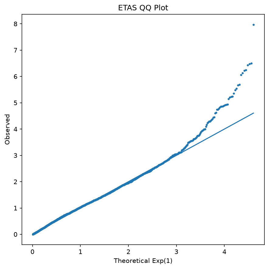
Figure 6: QQ plot of ETAS time-rescaled residuals against \(\text{Exp}(1)\). Points track the diagonal closely through most of the range, with the upper tail (largest residuals, corresponding to the biggest earthquakes) departing from the line — the residual model misspecification the KS test is picking up on.

Conclusion

The Hawkes process is a powerful tool for modeling event sequences where self-excitation matters. In seismology, it successfully captures earthquake clustering—a phenomenon that simple Poisson models completely miss.

Key takeaways:

1. Poisson processes are inadequate for most real-world clustered event data (earthquakes, disease outbreaks, neuron spikes, etc.)
2. Hawkes processes add minimal complexity but capture rich temporal structure
3. Self-excitation is ubiquitous: earthquakes trigger aftershocks; disease cases trigger new infections; one event reliably raises the odds of another
4. Inference is tractable: numerical optimization on log-likelihood works well in practice

For practitioners: If you observe clustering in your temporal data, try fitting a Hawkes process. The likelihood improvement over Poisson is often dramatic.

Further Reading

• A.G. Hawkes (1971) – Original self-exciting process paper
• Y. Ogata (1988) – Thinning algorithm for simulation
• A. Saichev & D. Sornette (2010) – ETAS in seismology
• Repository – https://github.com/fgias/earthquakes_hawkes